Intro to R
Module 5: The wonders of Purrr
TBD
Materials
Scripts
Click here to download the script! Save the script to the project directory you set up in the previous module.
Load your script in RStudio. To do this, open RStudio and click on the folder icon in the toolbar at the top to load your script.
Iteration
Often times you will want to apply the same function or multiple functions to multiple objects or inputs this is called iteration. In Base R, iterations are achieved by using for-loops, which are cumbersome and not very intuitive. If you’ve taken an R class before and covered for-loops, you are probably already nervous. But do not fear Tidyverse has made a package to conduct iteration operations that is much more user-friendly… and it has a cute inviting name, Purrr

Let’s go through a few examples of how the Purrr package can be used
Purrr map
As you can see from the Purrr cheat sheet, the Purrr package has a lot of usages. For the purposes of this course we will just be skimming the surface and mostly focus on applying functions with Purrr (upper left).
To apply the same function/s to a number of
objects we use the map()
function.
Let’s go through an example WITHOUT using Purrr first and then apply the tidyverse alternative.
Intro to purrr
First let’s generate a few random objects for us to work with
test_object_1 <- c(1:10)

test_object_2 <- c(11:20)

test_object_3 <- c(21:30)
We just generated three vectors of 10 numbers each
Now let’s say we want to extract the mean from each of these
The non-purrr way would be as follows
# for first object
mean(test_object_1)
## [1] 5.5# object 2
mean(test_object_2)## [1] 15.5# object 3
mean(test_object_2)## [1] 15.5While relatively easy to do, you can imagine if you had many more objects to work with, copy and pasting this code would get annoying and likely to produce errors the more times you have to do it.
Instead we can use Purrr to calculate the mean of all the objects at once
#first supply all the objects in a list
list(test_object_1,
     test_object_2,
     test_object_3) %>%

  # then use the map function with ~.x as a placeholder for all the objects before the last pipe (similar to '.')
  map(~.x %>%

        # then supply the function/s
        mean())
## [[1]]
## [1] 5.5
##
## [[2]]
## [1] 15.5
##
## [[3]]
## [1] 25.5Viola!
###The purrr process
Using Purrr might seem confusing at first, but it becomes second-hand nature once you have some practice, and by following these simple steps.
- First, write out the code you would use to perform the desired operation for A single object
- Second, ensure that this code is formatted in a dplyr pipe style code chunk (e.g., supply the object first, followed by a pipe for each operation you wish to perform on the supplied object ) AND est that this produces the desired outcome with a single object
- Supply a list of objects AND transfer all of your piped
functions inside of the purrr
map()function, providing ~.x as a placeholder for your list (If only one operation is being applied you can use ~function(.x) instead. I’ll show you both approaches
Let’s try this process for a simple object manipulation
Step 1
# code for one object
mean(test_object_1)
## [1] 5.5Step 2
# now let's adjust this code so it's in a dplyr pipe format
test_object_1 %>%

  mean()
## [1] 5.5This step is crucial! If your existing code isn’t already in dplyr format it will be much more difficult to transition to purrr
Step 3
# instead of one object we supply a list
list(test_object_1,
     test_object_2,
     test_object_3) %>%

  # then use the map function with ~.x as a placeholder for all the objects before the last pipe (similar to '.')
  map(~.x %>%

        # then supply the function/s
        mean())
## [[1]]
## [1] 5.5
##
## [[2]]
## [1] 15.5
##
## [[3]]
## [1] 25.5Import data with Purrr
One of the most common ways I use Purrr is when I want to read in multiple data sets for the same analysis. Often times landscape data, weather data, species data, etc. will be entered separately but you need all the data files for an analysis. Importing data with purrr isn’t as straighforward as other operations because there it isn’t intuitive how to accomplish step 2.
Start by reading in the 3 bobcat data files for this module, leave them named as they are
bobcat_collection_data <- read_csv('data/raw/bobcat_collection_data.csv')## Rows: 121 Columns: 7
## ── Column specification ────────────────────────────────────────────────────────
## Delimiter: ","
## chr (4): Bobcat_ID#, County, Township, CollectionDate
## dbl (3): Month, Coordinates_N, Coordinates_W
##
## ℹ Use `spec()` to retrieve the full column specification for this data.
## ℹ Specify the column types or set `show_col_types = FALSE` to quiet this message.bobcat_necropsy_data <- read_csv('data/raw/bobcat_necropsy_only_data.csv')## Rows: 121 Columns: 14
## ── Column specification ────────────────────────────────────────────────────────
## Delimiter: ","
## chr (13): Bobcat_ID#, NecropsyDate, Dissector, ApproxAge, Sex, Fecundity_Fem...
## dbl (1): Necropsy
##
## ℹ Use `spec()` to retrieve the full column specification for this data.
## ℹ Specify the column types or set `show_col_types = FALSE` to quiet this message.bobcat_age_data <- read_csv('data/raw/bobcat_age_data.csv')## Rows: 121 Columns: 2
## ── Column specification ────────────────────────────────────────────────────────
## Delimiter: ","
## chr (2): Bobcat_ID#, Age
##
## ℹ Use `spec()` to retrieve the full column specification for this data.
## ℹ Specify the column types or set `show_col_types = FALSE` to quiet this message.Now lets do this using Purrr!
First we need to assign our object to the environment with a name. When we read in multiple data frames at a time they will be stored in a list object. Lists can be confusing to work with at first but they follow a similar structure to a data frame. Let’s name this list bobcat_data.
And just like when we read in an individual data frame we need to provide the path for the data and the name and file extension (e.g. .csv, .txt.)
Then we were reference our purrr::map function AND the function we want to apply to all of the data. This is where things can get a bit confusing at first,
- Inside the parentheses for for the purrr::map
function we will reference the
read_csv()fuction, BUT we must preface this fuction with a ‘~’. The ‘~’ is part of the syntax Purrr uses. - Then where we would normally put the data file name we can substitute ‘.x’ which will reference the data in the list we already provided. Similar to the ‘.’ when using dplyr.
Let’s look at an example
# assign objects as list provide the names and file path of each data frame
bobcat_data <- list('data/raw/bobcat_collection_data.csv',
'data/raw/bobcat_necropsy_only_data.csv',
'data/raw/bobcat_age_data.csv') %>%
# use purrr::map to read in all data at once
purrr::map(
# this is alternative syntax you might see when only working with one function where the function is supplied after the '~' and '.x' is included in the function ()
~read_csv(.x)
)## Rows: 121 Columns: 7
## ── Column specification ────────────────────────────────────────────────────────
## Delimiter: ","
## chr (4): Bobcat_ID#, County, Township, CollectionDate
## dbl (3): Month, Coordinates_N, Coordinates_W
##
## ℹ Use `spec()` to retrieve the full column specification for this data.
## ℹ Specify the column types or set `show_col_types = FALSE` to quiet this message.
## Rows: 121 Columns: 14
## ── Column specification ────────────────────────────────────────────────────────
## Delimiter: ","
## chr (13): Bobcat_ID#, NecropsyDate, Dissector, ApproxAge, Sex, Fecundity_Fem...
## dbl  (1): Necropsy
##
## ℹ Use `spec()` to retrieve the full column specification for this data.
## ℹ Specify the column types or set `show_col_types = FALSE` to quiet this message.
## Rows: 121 Columns: 2
## ── Column specification ────────────────────────────────────────────────────────
## Delimiter: ","
## chr (2): Bobcat_ID#, Age
##
## ℹ Use `spec()` to retrieve the full column specification for this data.
## ℹ Specify the column types or set `show_col_types = FALSE` to quiet this message.# look at the list structure
str(bobcat_data)## List of 3
## $ : spc_tbl_ [121 × 7] (S3: spec_tbl_df/tbl_df/tbl/data.frame)
## ..$ Bobcat_ID# : chr [1:121] "5/18/01" "5/18/02" "58-18-03" "64-19-04" ...
## ..$ County : chr [1:121] "Athens" "Athens" "Morgan" "Perry" ...
## ..$ Township : chr [1:121] "Dover" "Canaan" "Hower" "Reading" ...
## ..$ CollectionDate: chr [1:121] "12/30/18" "12/14/18" "12/7/18" "2/10/19" ...
## ..$ Month : num [1:121] 12 12 12 2 1 3 2 2 2 3 ...
## ..$ Coordinates_N : num [1:121] 39.4 39.3 39.5 39.8 40.4 ...
## ..$ Coordinates_W : num [1:121] -82.1 -82 -82 -82.3 -81.2 ...
## ..- attr(*, "spec")=
## .. .. cols(
## .. .. `Bobcat_ID#` = col_character(),
## .. .. County = col_character(),
## .. .. Township = col_character(),
## .. .. CollectionDate = col_character(),
## .. .. Month = col_double(),
## .. .. Coordinates_N = col_double(),
## .. .. Coordinates_W = col_double()
## .. .. )
## ..- attr(*, "problems")=<externalptr>
## $ : spc_tbl_ [121 × 14] (S3: spec_tbl_df/tbl_df/tbl/data.frame)
## ..$ Bobcat_ID# : chr [1:121] "5/18/01" "5/18/02" "58-18-03" "64-19-04" ...
## ..$ Necropsy : num [1:121] 1 2 3 4 5 6 7 8 9 10 ...
## ..$ NecropsyDate : chr [1:121] "3/6/19" "3/9/19" "3/10/19" "3/13/19" ...
## ..$ Dissector : chr [1:121] "SP,_MD" "SP_MD_CH" "MD_CH" "MD_CH_HK" ...
## ..$ ApproxAge : chr [1:121] "Ad" "Ad" "Ad" "Juv" ...
## ..$ Sex : chr [1:121] "M" "F" "M" "F" ...
## ..$ Fecundity_Females: chr [1:121] "na" "na" "na" "0" ...
## ..$ RearFoot_cm : chr [1:121] "17.9" "16" "17.1" "14.7" ...
## ..$ Tail_cm : chr [1:121] "11.5" "11.5" "11.4" "11.3" ...
## ..$ Ear_cm : chr [1:121] "6.5" "6.5" "6.4" "6.5" ...
## ..$ Body_w/Tail_cm : chr [1:121] "89.5" "82" "92" "71.5" ...
## ..$ Body : chr [1:121] "78" "70.5" "80.6" "60.2" ...
## ..$ Weight_kg : chr [1:121] "13.6" "6.33" "9.98" "4.62" ...
## ..$ Condition : chr [1:121] "17.43589744" "8.978723404" "12.382134" "7.674418605" ...
## ..- attr(*, "spec")=
## .. .. cols(
## .. .. `Bobcat_ID#` = col_character(),
## .. .. Necropsy = col_double(),
## .. .. NecropsyDate = col_character(),
## .. .. Dissector = col_character(),
## .. .. ApproxAge = col_character(),
## .. .. Sex = col_character(),
## .. .. Fecundity_Females = col_character(),
## .. .. RearFoot_cm = col_character(),
## .. .. Tail_cm = col_character(),
## .. .. Ear_cm = col_character(),
## .. .. `Body_w/Tail_cm` = col_character(),
## .. .. Body = col_character(),
## .. .. Weight_kg = col_character(),
## .. .. Condition = col_character()
## .. .. )
## ..- attr(*, "problems")=<externalptr>
## $ : spc_tbl_ [121 × 2] (S3: spec_tbl_df/tbl_df/tbl/data.frame)
## ..$ Bobcat_ID#: chr [1:121] "5/18/01" "5/18/02" "58-18-03" "64-19-04" ...
## ..$ Age : chr [1:121] "3" "1" "2" "0" ...
## ..- attr(*, "spec")=
## .. .. cols(
## .. .. `Bobcat_ID#` = col_character(),
## .. .. Age = col_character()
## .. .. )
## ..- attr(*, "problems")=<externalptr>We can reduce our typing even further from the earlier example since all of the data are stored in the same folder by referencing a file path.
# assign object name to environment and provide file path for the data
bobcat_data <- file.path('data/raw',

  # provide the names of each data frame
  c('bobcat_collection_data.csv',
    'bobcat_necropsy_only_data.csv',
    'bobcat_age_data.csv')) %>%

  # use purrr::map to read in all data at once
  purrr::map(
    ~read_csv(.x))
## Rows: 121 Columns: 7
## ── Column specification ────────────────────────────────────────────────────────
## Delimiter: ","
## chr (4): Bobcat_ID#, County, Township, CollectionDate
## dbl (3): Month, Coordinates_N, Coordinates_W
##
## ℹ Use `spec()` to retrieve the full column specification for this data.
## ℹ Specify the column types or set `show_col_types = FALSE` to quiet this message.
## Rows: 121 Columns: 14
## ── Column specification ────────────────────────────────────────────────────────
## Delimiter: ","
## chr (13): Bobcat_ID#, NecropsyDate, Dissector, ApproxAge, Sex, Fecundity_Fem...
## dbl (1): Necropsy
##
## ℹ Use `spec()` to retrieve the full column specification for this data.
## ℹ Specify the column types or set `show_col_types = FALSE` to quiet this message.
## Rows: 121 Columns: 2
## ── Column specification ────────────────────────────────────────────────────────
## Delimiter: ","
## chr (2): Bobcat_ID#, Age
##
## ℹ Use `spec()` to retrieve the full column specification for this data.
## ℹ Specify the column types or set `show_col_types = FALSE` to quiet this message.str(bobcat_data)## List of 3
## $ : spc_tbl_ [121 × 7] (S3: spec_tbl_df/tbl_df/tbl/data.frame)
## ..$ Bobcat_ID# : chr [1:121] "5/18/01" "5/18/02" "58-18-03" "64-19-04" ...
## ..$ County : chr [1:121] "Athens" "Athens" "Morgan" "Perry" ...
## ..$ Township : chr [1:121] "Dover" "Canaan" "Hower" "Reading" ...
## ..$ CollectionDate: chr [1:121] "12/30/18" "12/14/18" "12/7/18" "2/10/19" ...
## ..$ Month : num [1:121] 12 12 12 2 1 3 2 2 2 3 ...
## ..$ Coordinates_N : num [1:121] 39.4 39.3 39.5 39.8 40.4 ...
## ..$ Coordinates_W : num [1:121] -82.1 -82 -82 -82.3 -81.2 ...
## ..- attr(*, "spec")=
## .. .. cols(
## .. .. `Bobcat_ID#` = col_character(),
## .. .. County = col_character(),
## .. .. Township = col_character(),
## .. .. CollectionDate = col_character(),
## .. .. Month = col_double(),
## .. .. Coordinates_N = col_double(),
## .. .. Coordinates_W = col_double()
## .. .. )
## ..- attr(*, "problems")=<externalptr>
## $ : spc_tbl_ [121 × 14] (S3: spec_tbl_df/tbl_df/tbl/data.frame)
## ..$ Bobcat_ID# : chr [1:121] "5/18/01" "5/18/02" "58-18-03" "64-19-04" ...
## ..$ Necropsy : num [1:121] 1 2 3 4 5 6 7 8 9 10 ...
## ..$ NecropsyDate : chr [1:121] "3/6/19" "3/9/19" "3/10/19" "3/13/19" ...
## ..$ Dissector : chr [1:121] "SP,_MD" "SP_MD_CH" "MD_CH" "MD_CH_HK" ...
## ..$ ApproxAge : chr [1:121] "Ad" "Ad" "Ad" "Juv" ...
## ..$ Sex : chr [1:121] "M" "F" "M" "F" ...
## ..$ Fecundity_Females: chr [1:121] "na" "na" "na" "0" ...
## ..$ RearFoot_cm : chr [1:121] "17.9" "16" "17.1" "14.7" ...
## ..$ Tail_cm : chr [1:121] "11.5" "11.5" "11.4" "11.3" ...
## ..$ Ear_cm : chr [1:121] "6.5" "6.5" "6.4" "6.5" ...
## ..$ Body_w/Tail_cm : chr [1:121] "89.5" "82" "92" "71.5" ...
## ..$ Body : chr [1:121] "78" "70.5" "80.6" "60.2" ...
## ..$ Weight_kg : chr [1:121] "13.6" "6.33" "9.98" "4.62" ...
## ..$ Condition : chr [1:121] "17.43589744" "8.978723404" "12.382134" "7.674418605" ...
## ..- attr(*, "spec")=
## .. .. cols(
## .. .. `Bobcat_ID#` = col_character(),
## .. .. Necropsy = col_double(),
## .. .. NecropsyDate = col_character(),
## .. .. Dissector = col_character(),
## .. .. ApproxAge = col_character(),
## .. .. Sex = col_character(),
## .. .. Fecundity_Females = col_character(),
## .. .. RearFoot_cm = col_character(),
## .. .. Tail_cm = col_character(),
## .. .. Ear_cm = col_character(),
## .. .. `Body_w/Tail_cm` = col_character(),
## .. .. Body = col_character(),
## .. .. Weight_kg = col_character(),
## .. .. Condition = col_character()
## .. .. )
## ..- attr(*, "problems")=<externalptr>
## $ : spc_tbl_ [121 × 2] (S3: spec_tbl_df/tbl_df/tbl/data.frame)
## ..$ Bobcat_ID#: chr [1:121] "5/18/01" "5/18/02" "58-18-03" "64-19-04" ...
## ..$ Age : chr [1:121] "3" "1" "2" "0" ...
## ..- attr(*, "spec")=
## .. .. cols(
## .. .. `Bobcat_ID#` = col_character(),
## .. .. Age = col_character()
## .. .. )
## ..- attr(*, "problems")=<externalptr>We could also format it like this if that makes more sense to you, using a period as the placeholder for the data file names
# assign object name to environment and provide list of data file names

bobcat_data <- list('bobcat_collection_data.csv',
                    'bobcat_necropsy_only_data.csv',
                    'bobcat_age_data.csv') %>%

  # provide file path for the data
  file.path('data/raw', .) %>%

  # use purrr::map to read in all data at once
  purrr::map(
    ~read_csv(.x))
## Rows: 121 Columns: 7
## ── Column specification ────────────────────────────────────────────────────────
## Delimiter: ","
## chr (4): Bobcat_ID#, County, Township, CollectionDate
## dbl (3): Month, Coordinates_N, Coordinates_W
##
## ℹ Use `spec()` to retrieve the full column specification for this data.
## ℹ Specify the column types or set `show_col_types = FALSE` to quiet this message.
## Rows: 121 Columns: 14
## ── Column specification ────────────────────────────────────────────────────────
## Delimiter: ","
## chr (13): Bobcat_ID#, NecropsyDate, Dissector, ApproxAge, Sex, Fecundity_Fem...
## dbl (1): Necropsy
##
## ℹ Use `spec()` to retrieve the full column specification for this data.
## ℹ Specify the column types or set `show_col_types = FALSE` to quiet this message.
## Rows: 121 Columns: 2
## ── Column specification ────────────────────────────────────────────────────────
## Delimiter: ","
## chr (2): Bobcat_ID#, Age
##
## ℹ Use `spec()` to retrieve the full column specification for this data.
## ℹ Specify the column types or set `show_col_types = FALSE` to quiet this message.str(bobcat_data)## List of 3
## $ : spc_tbl_ [121 × 7] (S3: spec_tbl_df/tbl_df/tbl/data.frame)
## ..$ Bobcat_ID# : chr [1:121] "5/18/01" "5/18/02" "58-18-03" "64-19-04" ...
## ..$ County : chr [1:121] "Athens" "Athens" "Morgan" "Perry" ...
## ..$ Township : chr [1:121] "Dover" "Canaan" "Hower" "Reading" ...
## ..$ CollectionDate: chr [1:121] "12/30/18" "12/14/18" "12/7/18" "2/10/19" ...
## ..$ Month : num [1:121] 12 12 12 2 1 3 2 2 2 3 ...
## ..$ Coordinates_N : num [1:121] 39.4 39.3 39.5 39.8 40.4 ...
## ..$ Coordinates_W : num [1:121] -82.1 -82 -82 -82.3 -81.2 ...
## ..- attr(*, "spec")=
## .. .. cols(
## .. .. `Bobcat_ID#` = col_character(),
## .. .. County = col_character(),
## .. .. Township = col_character(),
## .. .. CollectionDate = col_character(),
## .. .. Month = col_double(),
## .. .. Coordinates_N = col_double(),
## .. .. Coordinates_W = col_double()
## .. .. )
## ..- attr(*, "problems")=<externalptr>
## $ : spc_tbl_ [121 × 14] (S3: spec_tbl_df/tbl_df/tbl/data.frame)
## ..$ Bobcat_ID# : chr [1:121] "5/18/01" "5/18/02" "58-18-03" "64-19-04" ...
## ..$ Necropsy : num [1:121] 1 2 3 4 5 6 7 8 9 10 ...
## ..$ NecropsyDate : chr [1:121] "3/6/19" "3/9/19" "3/10/19" "3/13/19" ...
## ..$ Dissector : chr [1:121] "SP,_MD" "SP_MD_CH" "MD_CH" "MD_CH_HK" ...
## ..$ ApproxAge : chr [1:121] "Ad" "Ad" "Ad" "Juv" ...
## ..$ Sex : chr [1:121] "M" "F" "M" "F" ...
## ..$ Fecundity_Females: chr [1:121] "na" "na" "na" "0" ...
## ..$ RearFoot_cm : chr [1:121] "17.9" "16" "17.1" "14.7" ...
## ..$ Tail_cm : chr [1:121] "11.5" "11.5" "11.4" "11.3" ...
## ..$ Ear_cm : chr [1:121] "6.5" "6.5" "6.4" "6.5" ...
## ..$ Body_w/Tail_cm : chr [1:121] "89.5" "82" "92" "71.5" ...
## ..$ Body : chr [1:121] "78" "70.5" "80.6" "60.2" ...
## ..$ Weight_kg : chr [1:121] "13.6" "6.33" "9.98" "4.62" ...
## ..$ Condition : chr [1:121] "17.43589744" "8.978723404" "12.382134" "7.674418605" ...
## ..- attr(*, "spec")=
## .. .. cols(
## .. .. `Bobcat_ID#` = col_character(),
## .. .. Necropsy = col_double(),
## .. .. NecropsyDate = col_character(),
## .. .. Dissector = col_character(),
## .. .. ApproxAge = col_character(),
## .. .. Sex = col_character(),
## .. .. Fecundity_Females = col_character(),
## .. .. RearFoot_cm = col_character(),
## .. .. Tail_cm = col_character(),
## .. .. Ear_cm = col_character(),
## .. .. `Body_w/Tail_cm` = col_character(),
## .. .. Body = col_character(),
## .. .. Weight_kg = col_character(),
## .. .. Condition = col_character()
## .. .. )
## ..- attr(*, "problems")=<externalptr>
## $ : spc_tbl_ [121 × 2] (S3: spec_tbl_df/tbl_df/tbl/data.frame)
## ..$ Bobcat_ID#: chr [1:121] "5/18/01" "5/18/02" "58-18-03" "64-19-04" ...
## ..$ Age : chr [1:121] "3" "1" "2" "0" ...
## ..- attr(*, "spec")=
## .. .. cols(
## .. .. `Bobcat_ID#` = col_character(),
## .. .. Age = col_character()
## .. .. )
## ..- attr(*, "problems")=<externalptr>We can look at each list element by using the
$ similar to a data frame.
Let’s see what are list elements are named using the
names() argument.
# first see what the list elements are named
names(bobcat_data)
## NULLhmmmm that’s not ideal, our list elements don’t have names. We can
fix this by adding a function outside the
Purrrr::map() to rename each object in the list.
# assign object name to environment and provide file path for the data
bobcat_data <- file.path('data/raw',

  # provide the names of each data frame
  c('bobcat_collection_data.csv',
    'bobcat_necropsy_only_data.csv',
    'bobcat_age_data.csv')) %>%

  # use purrr::map to read in all data at once
  purrr::map(
    ~read_csv(.x)) %>%

  # assign names to list objects
purrr::set_names('collection',
                   'necropsy',
                   'age')
## Rows: 121 Columns: 7
## ── Column specification ────────────────────────────────────────────────────────
## Delimiter: ","
## chr (4): Bobcat_ID#, County, Township, CollectionDate
## dbl (3): Month, Coordinates_N, Coordinates_W
##
## ℹ Use `spec()` to retrieve the full column specification for this data.
## ℹ Specify the column types or set `show_col_types = FALSE` to quiet this message.
## Rows: 121 Columns: 14
## ── Column specification ────────────────────────────────────────────────────────
## Delimiter: ","
## chr (13): Bobcat_ID#, NecropsyDate, Dissector, ApproxAge, Sex, Fecundity_Fem...
## dbl (1): Necropsy
##
## ℹ Use `spec()` to retrieve the full column specification for this data.
## ℹ Specify the column types or set `show_col_types = FALSE` to quiet this message.
## Rows: 121 Columns: 2
## ── Column specification ────────────────────────────────────────────────────────
## Delimiter: ","
## chr (2): Bobcat_ID#, Age
##
## ℹ Use `spec()` to retrieve the full column specification for this data.
## ℹ Specify the column types or set `show_col_types = FALSE` to quiet this message.str(bobcat_data)## List of 3
## $ collection: spc_tbl_ [121 × 7] (S3: spec_tbl_df/tbl_df/tbl/data.frame)
## ..$ Bobcat_ID# : chr [1:121] "5/18/01" "5/18/02" "58-18-03" "64-19-04" ...
## ..$ County : chr [1:121] "Athens" "Athens" "Morgan" "Perry" ...
## ..$ Township : chr [1:121] "Dover" "Canaan" "Hower" "Reading" ...
## ..$ CollectionDate: chr [1:121] "12/30/18" "12/14/18" "12/7/18" "2/10/19" ...
## ..$ Month : num [1:121] 12 12 12 2 1 3 2 2 2 3 ...
## ..$ Coordinates_N : num [1:121] 39.4 39.3 39.5 39.8 40.4 ...
## ..$ Coordinates_W : num [1:121] -82.1 -82 -82 -82.3 -81.2 ...
## ..- attr(*, "spec")=
## .. .. cols(
## .. .. `Bobcat_ID#` = col_character(),
## .. .. County = col_character(),
## .. .. Township = col_character(),
## .. .. CollectionDate = col_character(),
## .. .. Month = col_double(),
## .. .. Coordinates_N = col_double(),
## .. .. Coordinates_W = col_double()
## .. .. )
## ..- attr(*, "problems")=<externalptr>
## $ necropsy : spc_tbl_ [121 × 14] (S3: spec_tbl_df/tbl_df/tbl/data.frame)
## ..$ Bobcat_ID# : chr [1:121] "5/18/01" "5/18/02" "58-18-03" "64-19-04" ...
## ..$ Necropsy : num [1:121] 1 2 3 4 5 6 7 8 9 10 ...
## ..$ NecropsyDate : chr [1:121] "3/6/19" "3/9/19" "3/10/19" "3/13/19" ...
## ..$ Dissector : chr [1:121] "SP,_MD" "SP_MD_CH" "MD_CH" "MD_CH_HK" ...
## ..$ ApproxAge : chr [1:121] "Ad" "Ad" "Ad" "Juv" ...
## ..$ Sex : chr [1:121] "M" "F" "M" "F" ...
## ..$ Fecundity_Females: chr [1:121] "na" "na" "na" "0" ...
## ..$ RearFoot_cm : chr [1:121] "17.9" "16" "17.1" "14.7" ...
## ..$ Tail_cm : chr [1:121] "11.5" "11.5" "11.4" "11.3" ...
## ..$ Ear_cm : chr [1:121] "6.5" "6.5" "6.4" "6.5" ...
## ..$ Body_w/Tail_cm : chr [1:121] "89.5" "82" "92" "71.5" ...
## ..$ Body : chr [1:121] "78" "70.5" "80.6" "60.2" ...
## ..$ Weight_kg : chr [1:121] "13.6" "6.33" "9.98" "4.62" ...
## ..$ Condition : chr [1:121] "17.43589744" "8.978723404" "12.382134" "7.674418605" ...
## ..- attr(*, "spec")=
## .. .. cols(
## .. .. `Bobcat_ID#` = col_character(),
## .. .. Necropsy = col_double(),
## .. .. NecropsyDate = col_character(),
## .. .. Dissector = col_character(),
## .. .. ApproxAge = col_character(),
## .. .. Sex = col_character(),
## .. .. Fecundity_Females = col_character(),
## .. .. RearFoot_cm = col_character(),
## .. .. Tail_cm = col_character(),
## .. .. Ear_cm = col_character(),
## .. .. `Body_w/Tail_cm` = col_character(),
## .. .. Body = col_character(),
## .. .. Weight_kg = col_character(),
## .. .. Condition = col_character()
## .. .. )
## ..- attr(*, "problems")=<externalptr>
## $ age : spc_tbl_ [121 × 2] (S3: spec_tbl_df/tbl_df/tbl/data.frame)
## ..$ Bobcat_ID#: chr [1:121] "5/18/01" "5/18/02" "58-18-03" "64-19-04" ...
## ..$ Age : chr [1:121] "3" "1" "2" "0" ...
## ..- attr(*, "spec")=
## .. .. cols(
## .. .. `Bobcat_ID#` = col_character(),
## .. .. Age = col_character()
## .. .. )
## ..- attr(*, "problems")=<externalptr>Now we can look at each list element like by using
the $
# look at the structure of the necropsy data
str(bobcat_data$necropsy)
## spc_tbl_ [121 × 14] (S3: spec_tbl_df/tbl_df/tbl/data.frame)
## $ Bobcat_ID# : chr [1:121] "5/18/01" "5/18/02" "58-18-03" "64-19-04" ...
## $ Necropsy : num [1:121] 1 2 3 4 5 6 7 8 9 10 ...
## $ NecropsyDate : chr [1:121] "3/6/19" "3/9/19" "3/10/19" "3/13/19" ...
## $ Dissector : chr [1:121] "SP,_MD" "SP_MD_CH" "MD_CH" "MD_CH_HK" ...
## $ ApproxAge : chr [1:121] "Ad" "Ad" "Ad" "Juv" ...
## $ Sex : chr [1:121] "M" "F" "M" "F" ...
## $ Fecundity_Females: chr [1:121] "na" "na" "na" "0" ...
## $ RearFoot_cm : chr [1:121] "17.9" "16" "17.1" "14.7" ...
## $ Tail_cm : chr [1:121] "11.5" "11.5" "11.4" "11.3" ...
## $ Ear_cm : chr [1:121] "6.5" "6.5" "6.4" "6.5" ...
## $ Body_w/Tail_cm : chr [1:121] "89.5" "82" "92" "71.5" ...
## $ Body : chr [1:121] "78" "70.5" "80.6" "60.2" ...
## $ Weight_kg : chr [1:121] "13.6" "6.33" "9.98" "4.62" ...
## $ Condition : chr [1:121] "17.43589744" "8.978723404" "12.382134" "7.674418605" ...
## - attr(*, "spec")=
## .. cols(
## .. `Bobcat_ID#` = col_character(),
## .. Necropsy = col_double(),
## .. NecropsyDate = col_character(),
## .. Dissector = col_character(),
## .. ApproxAge = col_character(),
## .. Sex = col_character(),
## .. Fecundity_Females = col_character(),
## .. RearFoot_cm = col_character(),
## .. Tail_cm = col_character(),
## .. Ear_cm = col_character(),
## .. `Body_w/Tail_cm` = col_character(),
## .. Body = col_character(),
## .. Weight_kg = col_character(),
## .. Condition = col_character()
## .. )
## - attr(*, "problems")=<externalptr>Many of the columns read in improperly, we could tackle this
individually for each dataframe, or we could include specification for
the various column types in our map() function.
# assign object name to environment and provide file path for the data
bobcat_data <- file.path('data/raw',

  # provide the names of each data frame
  c('bobcat_collection_data.csv',
    'bobcat_necropsy_only_data.csv',
    'bobcat_age_data.csv')) %>%

  # use purrr::map to read in all data at once
  purrr::map(
    ~read_csv(.x,

              col_types = cols(RearFoot_cm = col_number(),
                                  Tail_cm = col_number(),
                                  Ear_cm = col_number(),
                                  'Body_w/Tail_cm' = col_number(),
                                  Body = col_number(),
                                  Weight_kg = col_number(),
                                  Condition = col_number(),
                               Age = col_number(),
                       .default = col_factor())
              )) %>%

  # assign names to list objects
purrr::set_names('collection',
                   'necropsy',
                   'age')

str(bobcat_data$necropsy)
## spc_tbl_ [121 × 14] (S3: spec_tbl_df/tbl_df/tbl/data.frame)
## $ Bobcat_ID# : Factor w/ 121 levels "5/18/01","5/18/02",..: 1 2 3 4 5 6 7 8 9 10 ...
## $ Necropsy : Factor w/ 121 levels "1","2","3","4",..: 1 2 3 4 5 6 7 8 9 10 ...
## $ NecropsyDate : Factor w/ 68 levels "3/6/19","3/9/19",..: 1 2 3 4 5 6 7 8 9 10 ...
## $ Dissector : Factor w/ 35 levels "SP,_MD","SP_MD_CH",..: 1 2 3 4 5 3 6 4 3 6 ...
## $ ApproxAge : Factor w/ 4 levels "Ad","Juv","na",..: 1 1 1 2 1 1 1 1 2 1 ...
## $ Sex : Factor w/ 3 levels "M","F","na": 1 2 1 2 1 1 1 1 1 1 ...
## $ Fecundity_Females: Factor w/ 7 levels "na","0","2","4",..: 1 1 1 2 1 1 1 1 1 1 ...
## $ RearFoot_cm : num [1:121] 17.9 16 17.1 14.7 16.5 16 17 18.2 14.6 16.4 ...
## $ Tail_cm : num [1:121] 11.5 11.5 11.4 11.3 14 12.5 12.5 13 10 14.5 ...
## $ Ear_cm : num [1:121] 6.5 6.5 6.4 6.5 5.7 6.5 7 6.5 7 7.2 ...
## $ Body_w/Tail_cm : num [1:121] 89.5 82 92 71.5 95.2 ...
## $ Body : num [1:121] 78 70.5 80.6 60.2 81.2 ...
## $ Weight_kg : num [1:121] 13.6 6.33 9.98 4.62 11.53 ...
## $ Condition : num [1:121] 17.44 8.98 12.38 7.67 14.19 ...
## - attr(*, "spec")=
## .. cols(
## .. .default = col_factor(),
## .. `Bobcat_ID#` = col_factor(levels = NULL, ordered = FALSE, include_na = FALSE),
## .. Necropsy = col_factor(levels = NULL, ordered = FALSE, include_na = FALSE),
## .. NecropsyDate = col_factor(levels = NULL, ordered = FALSE, include_na = FALSE),
## .. Dissector = col_factor(levels = NULL, ordered = FALSE, include_na = FALSE),
## .. ApproxAge = col_factor(levels = NULL, ordered = FALSE, include_na = FALSE),
## .. Sex = col_factor(levels = NULL, ordered = FALSE, include_na = FALSE),
## .. Fecundity_Females = col_factor(levels = NULL, ordered = FALSE, include_na = FALSE),
## .. RearFoot_cm = col_number(),
## .. Tail_cm = col_number(),
## .. Ear_cm = col_number(),
## .. `Body_w/Tail_cm` = col_number(),
## .. Body = col_number(),
## .. Weight_kg = col_number(),
## .. Condition = col_number()
## .. )
## - attr(*, "problems")=<externalptr>If your data frames don’t have all the same names of columns, which they usually don’t, you will likely get a warning about parsing issues. You can ignore this just be sure to check the structure of each dataframe in your list before proceeding and ensure the variables you need later read in properly.
Format/manipulate data with Purrr
We can also use Purrr to manipulate our data. Recall I recommend always using lowercase for column names, objects, etc. The bobcat data when entered does not follow those rules so we’d want to change that after we import in R.
Let’s look at the non-purrr way first and then see how much code repetition we avoid when we use Purrr. We would likely want to do this when we read in the data so, on your own copy the non-purrr code from above where we read in the data, and set the column names to lowercase for each data set.
Use the head() function to
look at the first few rows of each data
set.
bobcat_collection_data <- read_csv('data/raw/bobcat_collection_data.csv') %>%

  # set names to lowercase
  set_names(
    names(.) %>%
      tolower())
## Rows: 121 Columns: 7
## ── Column specification ────────────────────────────────────────────────────────
## Delimiter: ","
## chr (4): Bobcat_ID#, County, Township, CollectionDate
## dbl (3): Month, Coordinates_N, Coordinates_W
##
## ℹ Use `spec()` to retrieve the full column specification for this data.
## ℹ Specify the column types or set `show_col_types = FALSE` to quiet this message.head(bobcat_collection_data)## # A tibble: 6 × 7
## `bobcat_id#` county township collectiondate month coordinates_n coordinates_w
## <chr> <chr> <chr> <chr> <dbl> <dbl> <dbl>
## 1 5/18/01 Athens Dover 12/30/18 12 39.4 -82.1
## 2 5/18/02 Athens Canaan 12/14/18 12 39.3 -82.0
## 3 58-18-03 Morgan Hower 12/7/18 12 39.5 -82.0
## 4 64-19-04 Perry Reading 2/10/19 2 39.8 -82.3
## 5 34-15-05 Harris… Monroe 1/11/15 1 40.4 -81.2
## 6 71-19-06 Ross Jeffers… 3/7/19 3 39.2 -82.8bobcat_necropsy_data <- read_csv('data/raw/bobcat_necropsy_only_data.csv')%>%
# set names to lowercase
set_names(
names(.) %>%
tolower())## Rows: 121 Columns: 14
## ── Column specification ────────────────────────────────────────────────────────
## Delimiter: ","
## chr (13): Bobcat_ID#, NecropsyDate, Dissector, ApproxAge, Sex, Fecundity_Fem...
## dbl (1): Necropsy
##
## ℹ Use `spec()` to retrieve the full column specification for this data.
## ℹ Specify the column types or set `show_col_types = FALSE` to quiet this message.head(bobcat_necropsy_data)## # A tibble: 6 × 14
## `bobcat_id#` necropsy necropsydate dissector approxage sex fecundity_females
## <chr> <dbl> <chr> <chr> <chr> <chr> <chr>
## 1 5/18/01 1 3/6/19 SP,_MD Ad M na
## 2 5/18/02 2 3/9/19 SP_MD_CH Ad F na
## 3 58-18-03 3 3/10/19 MD_CH Ad M na
## 4 64-19-04 4 3/13/19 MD_CH_HK Juv F 0
## 5 34-15-05 5 3/23/19 MD_CH_JG Ad M na
## 6 71-19-06 6 3/24/19 MD_CH Ad M na
## # ℹ 7 more variables: rearfoot_cm <chr>, tail_cm <chr>, ear_cm <chr>,
## # `body_w/tail_cm` <chr>, body <chr>, weight_kg <chr>, condition <chr>bobcat_age_data <- read_csv('data/raw/bobcat_age_data.csv')%>%
# set names to lowercase
set_names(
names(.) %>%
tolower())## Rows: 121 Columns: 2
## ── Column specification ────────────────────────────────────────────────────────
## Delimiter: ","
## chr (2): Bobcat_ID#, Age
##
## ℹ Use `spec()` to retrieve the full column specification for this data.
## ℹ Specify the column types or set `show_col_types = FALSE` to quiet this message.head(bobcat_age_data)## # A tibble: 6 × 2
## `bobcat_id#` age
## <chr> <chr>
## 1 5/18/01 3
## 2 5/18/02 1
## 3 58-18-03 2
## 4 64-19-04 0
## 5 34-15-05 1
## 6 71-19-06 XThat’s a lot of repetition in our code, which we generally want to avoid whenever possible. With Purrr we can do just that.
We are going to use the same code from above that we used to read in the data files using a file path, and we will add a function to set the column names to lower case.
To do multiple iterations within the same
purrr::map() function we have to change
one thing. Instead of typing a ‘~’ before the read_csv()
function and referencing our list (.x) inside the
read_csv() function we need to reference
the list elements first and then supply the multiple
funcitons we want to apply.
See below
# assign object name to environment and provide file path for the data
bobcat_data <- file.path('data/raw',

                         # provide the names of each data frame
                         c('bobcat_collection_data.csv',
                           'bobcat_necropsy_only_data.csv',
                           'bobcat_age_data.csv')) %>%

  # use purrr::map to read in all data at once
  purrr::map(

    # reference list elements with ~
    ~.x %>%

      # read in list elements
      read_csv(col_types = cols(RearFoot_cm = col_number(),
                                  Tail_cm = col_number(),
                                  Ear_cm = col_number(),
                                  'Body_w/Tail_cm' = col_number(),
                                  Body = col_number(),
                                  Weight_kg = col_number(),
                                  Condition = col_number(),
                               Age = col_number(),
                       .default = col_factor())
            ) %>%

      # set names to lower case
      set_names(
        names(.) %>%
          tolower())
  ) %>%

  # assign names to list objects
purrr::set_names('collection',
                   'necropsy',
                   'age')
## Warning: The following named parsers don't match the column names: RearFoot_cm,
## Tail_cm, Ear_cm, Body_w/Tail_cm, Body, Weight_kg, Condition, Age## Warning: The following named parsers don't match the column names: Age## Warning: One or more parsing issues, call `problems()` on your data frame for details,
## e.g.:
## dat <- vroom(...)
## problems(dat)## Warning: The following named parsers don't match the column names: RearFoot_cm,
## Tail_cm, Ear_cm, Body_w/Tail_cm, Body, Weight_kg, Condition## Warning: One or more parsing issues, call `problems()` on your data frame for details,
## e.g.:
## dat <- vroom(...)
## problems(dat)head(bobcat_data$bobcat_collection)## NULLI also don’t like the column name for ‘bobcat ID number’. See how it reads in with ’’ because someone used the ‘#’ instead of typing number and R doesn’t like that. Let’s change this in all the data sets using Purrr.
For this example we won’t go through the non-purrr way to save time
# assign object name to environment and provide file path for the data
bobcat_data <- file.path('data/raw',

                         # provide the names of each data frame
                         c('bobcat_collection_data.csv',
                           'bobcat_necropsy_only_data.csv',
                           'bobcat_age_data.csv')) %>%

  # use purrr::map to read in all data at once
  purrr::map(

    # reference list elements with ~
    ~.x %>%

      # read in list elements
      read_csv(col_types = cols(RearFoot_cm = col_number(),
                                  Tail_cm = col_number(),
                                  Ear_cm = col_number(),
                                  'Body_w/Tail_cm' = col_number(),
                                  Body = col_number(),
                                  Weight_kg = col_number(),
                                  Condition = col_number(),
                               Age = col_number(),
                       .default = col_factor())
            ) %>%

      # set names to lower case
      set_names(
        names(.) %>%
          tolower()) %>%

      # change bobcats id# to better name
      rename(.,
             'bobcat_id' = 'bobcat_id#') # new name = old name
  ) %>%

  # assign names to list objects
  purrr::set_names('collection',
                   'necropsy',
                   'age')
## Warning: The following named parsers don't match the column names: RearFoot_cm,
## Tail_cm, Ear_cm, Body_w/Tail_cm, Body, Weight_kg, Condition, Age## Warning: The following named parsers don't match the column names: Age## Warning: One or more parsing issues, call `problems()` on your data frame for details,
## e.g.:
## dat <- vroom(...)
## problems(dat)## Warning: The following named parsers don't match the column names: RearFoot_cm,
## Tail_cm, Ear_cm, Body_w/Tail_cm, Body, Weight_kg, Condition## Warning: One or more parsing issues, call `problems()` on your data frame for details,
## e.g.:
## dat <- vroom(...)
## problems(dat)head(bobcat_data$collection)## # A tibble: 6 × 7
## bobcat_id county township collectiondate month coordinates_n coordinates_w
## <fct> <fct> <fct> <fct> <fct> <fct> <fct>
## 1 5/18/01 Athens Dover 12/30/18 12 39.38911 -82.14085
## 2 5/18/02 Athens Canaan 12/14/18 12 39.30614 -81.957962
## 3 58-18-03 Morgan Hower 12/7/18 12 39.494746 -81.988452
## 4 64-19-04 Perry Reading 2/10/19 2 39.822288 -82.286951
## 5 34-15-05 Harrison Monroe 1/11/15 1 40.420816 -81.216981
## 6 71-19-06 Ross Jefferson 3/7/19 3 39.23797 -82.7881Much better!
Purrr imap
Saving data
Now that we have tidy data sets we may want to save these to our hard drive so we don’t have to run code to reformat them every time we read in the data.
In your script, type code that will save each of the data sets in the bobcat_data list as a csv to the data/processed folder.
# save each data set as a csv
write_csv(bobcat_data$collection,
          'data/processed/bobcat_collection.csv')

write_csv(bobcat_data$age,
          'data/processed/bobcat_age.csv')

write_csv(bobcat_data$necropsy,
          'data/processed/bobcat_necropsy.csv')
Now the Purrr way!
We can use the Purrr function
imap() because it retains the names of elements within our
list (.y) when we save them
# save each data set as a csv
purrr::imap(
  bobcat_data,
  ~write_csv(.x,
             file = paste0("data/processed/",
                           .y,
                           '.csv')))
## $collection
## # A tibble: 121 × 7
## bobcat_id county township collectiondate month coordinates_n coordinates_w
## <fct> <fct> <fct> <fct> <fct> <fct> <fct>
## 1 5/18/01 Athens Dover 12/30/18 12 39.38911 -82.14085
## 2 5/18/02 Athens Canaan 12/14/18 12 39.30614 -81.957962
## 3 58-18-03 Morgan Hower 12/7/18 12 39.494746 -81.988452
## 4 64-19-04 Perry Reading 2/10/19 2 39.822288 -82.286951
## 5 34-15-05 Harrison Monroe 1/11/15 1 40.420816 -81.216981
## 6 71-19-06 Ross Jeffers… 3/7/19 3 39.23797 -82.7881
## 7 16-19-07 Coshocton Jeffers… 2/28/19 2 40.3524 -82.018
## 8 40-19-08 Jackson Madison 2/27/19 2 38.903 -82.4497
## 9 61-19-09 Noble Elk 2/20/19 2 39.65858 -81.28657
## 10 27-19-10 Gallia Gallipo… 3/1/19 3 38.8425 -82.1815
## # ℹ 111 more rows
##
## $necropsy
## # A tibble: 121 × 14
## bobcat_id necropsy necropsydate dissector approxage sex fecundity_females
## <fct> <fct> <fct> <fct> <fct> <fct> <fct>
## 1 5/18/01 1 3/6/19 SP,_MD Ad M na
## 2 5/18/02 2 3/9/19 SP_MD_CH Ad F na
## 3 58-18-03 3 3/10/19 MD_CH Ad M na
## 4 64-19-04 4 3/13/19 MD_CH_HK Juv F 0
## 5 34-15-05 5 3/23/19 MD_CH_JG Ad M na
## 6 71-19-06 6 3/24/19 MD_CH Ad M na
## 7 16-19-07 7 3/31/19 MD_HK Ad M na
## 8 40-19-08 8 4/7/19 MD_CH_HK Ad M na
## 9 61-19-09 9 4/13/19 MD_CH Juv M na
## 10 27-19-10 10 4/14/19 MD_HK Ad M na
## # ℹ 111 more rows
## # ℹ 7 more variables: rearfoot_cm <dbl>, tail_cm <dbl>, ear_cm <dbl>,
## # `body_w/tail_cm` <dbl>, body <dbl>, weight_kg <dbl>, condition <dbl>
##
## $age
## # A tibble: 121 × 2
## bobcat_id age
## <fct> <dbl>
## 1 5/18/01 3
## 2 5/18/02 1
## 3 58-18-03 2
## 4 64-19-04 0
## 5 34-15-05 1
## 6 71-19-06 NA
## 7 16-19-07 NA
## 8 40-19-08 1
## 9 61-19-09 0
## 10 27-19-10 3
## # ℹ 111 more rowsSo much less repetition and code if you have a lot of data sets to save
###Figures
If you’ve done assignment 4, you may have been annoyed with how much code repetition there was to generate all the histograms for your explanatory variables. But not to fear, Purrr is here!
We can use Purrr’s imap() function to quickly
generate several of the same plot without having to copy and paste a
bunch of code.
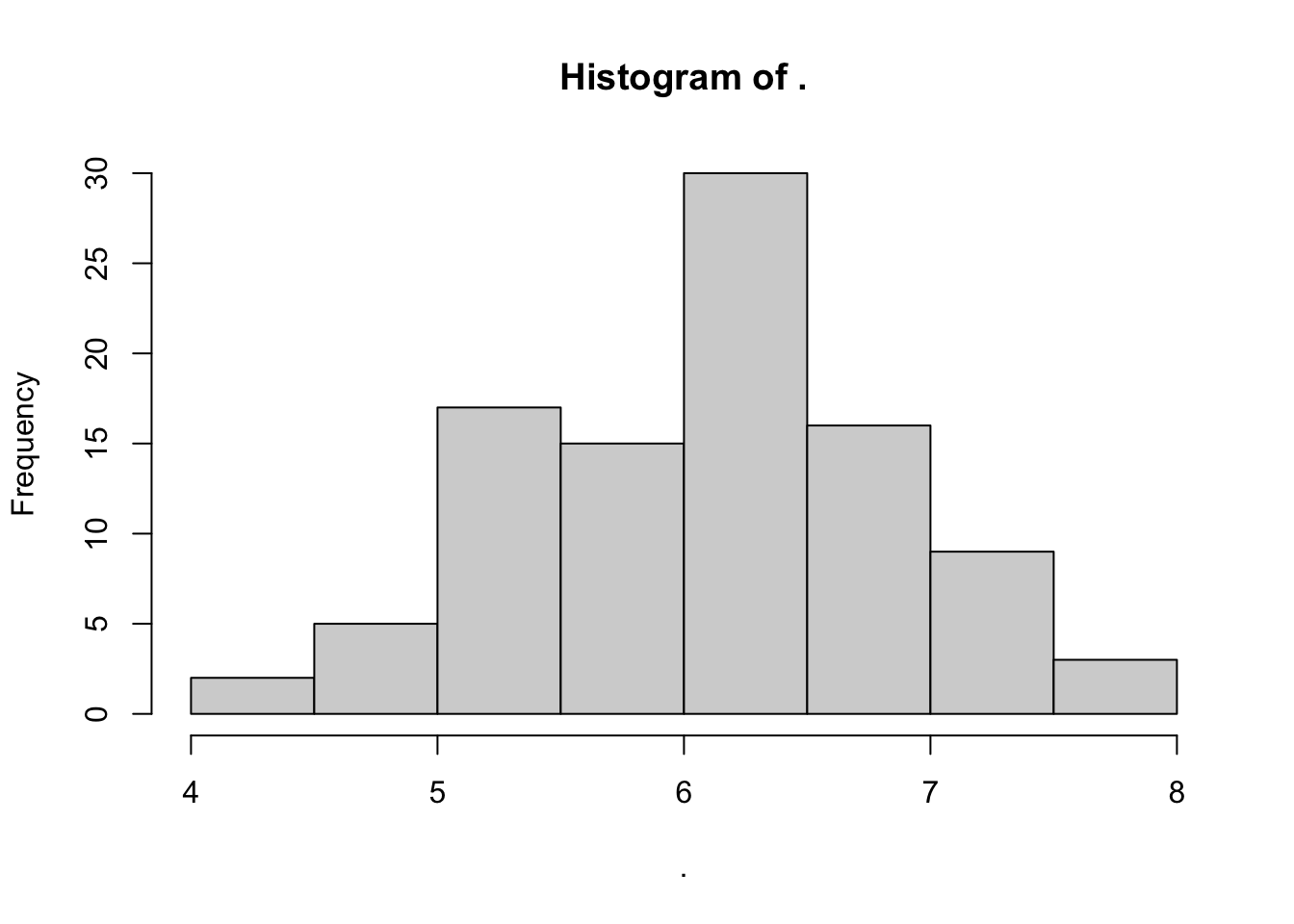
In your script attempt to make histograms for all the numeric variables in the necropsy data following the 3 steps I outlined earlier
# step 1: code for 1 histogram
hist(bobcat_data$necropsy$rearfoot_cm)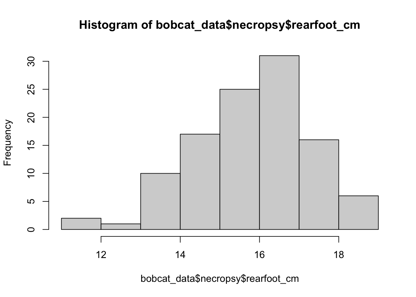
# step 2: translate code to dplyr pipe format
bobcat_data$necropsy$rearfoot_cm %>%

  hist()
# step 3: provide list and pipe into `map()`
bobcat_data$necropsy %>%

  # select only numeric vars
  select(is.numeric) %>%

  # apply purrr::map
  map(~.x %>%
        #provide histograms
        hist()
  )
## Warning: Use of bare predicate functions was deprecated in tidyselect 1.1.0.
## ℹ Please use wrap predicates in `where()` instead.
## # Was:
## data %>% select(is.numeric)
##
## # Now:
## data %>% select(where(is.numeric))
## This warning is displayed once every 8 hours.
## Call `lifecycle::last_lifecycle_warnings()` to see where this warning was
## generated.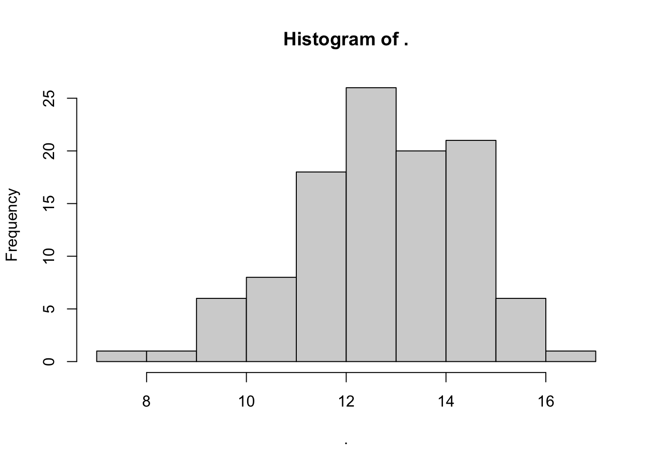
## $rearfoot_cm
## $breaks
## [1] 11 12 13 14 15 16 17 18 19
##
## $counts
## [1] 2 1 10 17 25 31 16 6
##
## $density
## [1] 0.018518519 0.009259259 0.092592593 0.157407407 0.231481481 0.287037037
## [7] 0.148148148 0.055555556
##
## $mids
## [1] 11.5 12.5 13.5 14.5 15.5 16.5 17.5 18.5
##
## $xname
## [1] "."
##
## $equidist
## [1] TRUE
##
## attr(,"class")
## [1] "histogram"
##
## $tail_cm
## $breaks
## [1] 7 8 9 10 11 12 13 14 15 16 17
##
## $counts
## [1] 1 1 6 8 18 26 20 21 6 1
##
## $density
## [1] 0.009259259 0.009259259 0.055555556 0.074074074 0.166666667 0.240740741
## [7] 0.185185185 0.194444444 0.055555556 0.009259259
##
## $mids
## [1] 7.5 8.5 9.5 10.5 11.5 12.5 13.5 14.5 15.5 16.5
##
## $xname
## [1] "."
##
## $equidist
## [1] TRUE
##
## attr(,"class")
## [1] "histogram"
##
## $ear_cm
## $breaks
## [1] 4.0 4.5 5.0 5.5 6.0 6.5 7.0 7.5 8.0
##
## $counts
## [1] 2 5 17 15 30 16 9 3
##
## $density
## [1] 0.04123711 0.10309278 0.35051546 0.30927835 0.61855670 0.32989691 0.18556701
## [8] 0.06185567
##
## $mids
## [1] 4.25 4.75 5.25 5.75 6.25 6.75 7.25 7.75
##
## $xname
## [1] "."
##
## $equidist
## [1] TRUE
##
## attr(,"class")
## [1] "histogram"
##
## $`body_w/tail_cm`
## $breaks
## [1] 55 60 65 70 75 80 85 90 95 100 105
##
## $counts
## [1] 3 2 5 14 22 20 23 13 5 1
##
## $density
## [1] 0.005555556 0.003703704 0.009259259 0.025925926 0.040740741 0.037037037
## [7] 0.042592593 0.024074074 0.009259259 0.001851852
##
## $mids
## [1] 57.5 62.5 67.5 72.5 77.5 82.5 87.5 92.5 97.5 102.5
##
## $xname
## [1] "."
##
## $equidist
## [1] TRUE
##
## attr(,"class")
## [1] "histogram"
##
## $body
## $breaks
## [1] 45 50 55 60 65 70 75 80 85 90
##
## $counts
## [1] 3 2 11 16 26 24 19 5 2
##
## $density
## [1] 0.005555556 0.003703704 0.020370370 0.029629630 0.048148148 0.044444444
## [7] 0.035185185 0.009259259 0.003703704
##
## $mids
## [1] 47.5 52.5 57.5 62.5 67.5 72.5 77.5 82.5 87.5
##
## $xname
## [1] "."
##
## $equidist
## [1] TRUE
##
## attr(,"class")
## [1] "histogram"
##
## $weight_kg
## $breaks
## [1] 0 2 4 6 8 10 12 14
##
## $counts
## [1] 2 10 27 31 24 9 5
##
## $density
## [1] 0.009259259 0.046296296 0.125000000 0.143518519 0.111111111 0.041666667
## [7] 0.023148148
##
## $mids
## [1] 1 3 5 7 9 11 13
##
## $xname
## [1] "."
##
## $equidist
## [1] TRUE
##
## attr(,"class")
## [1] "histogram"
##
## $condition
## $breaks
## [1] 2 4 6 8 10 12 14 16 18
##
## $counts
## [1] 1 9 17 26 25 20 6 4
##
## $density
## [1] 0.00462963 0.04166667 0.07870370 0.12037037 0.11574074 0.09259259 0.02777778
## [8] 0.01851852
##
## $mids
## [1] 3 5 7 9 11 13 15 17
##
## $xname
## [1] "."
##
## $equidist
## [1] TRUE
##
## attr(,"class")
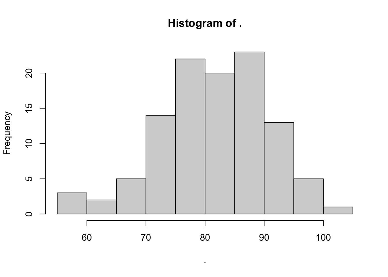
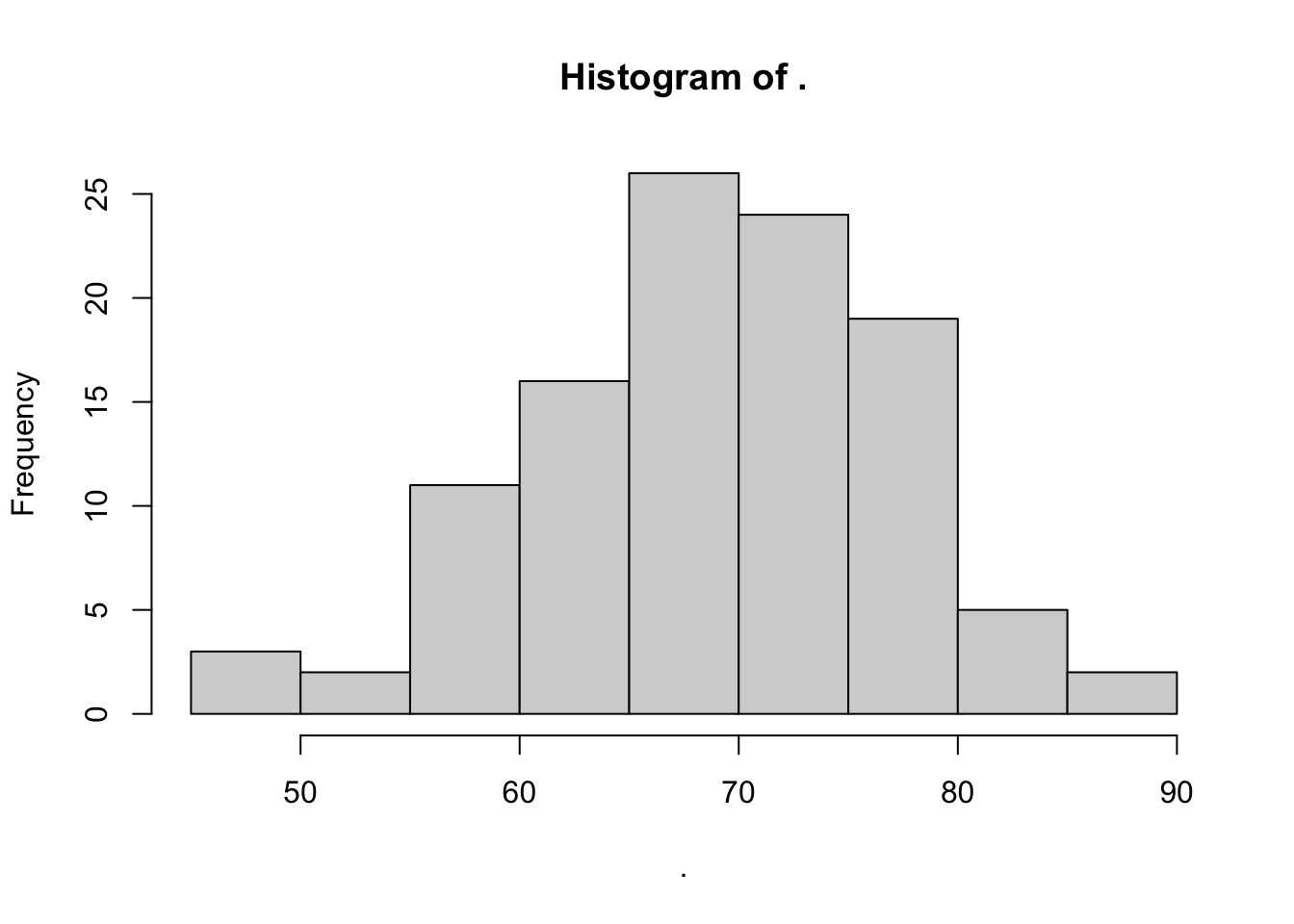
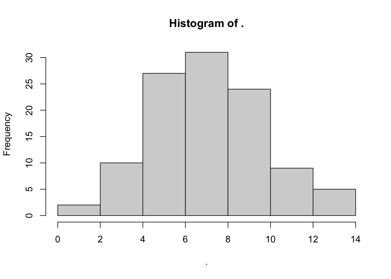
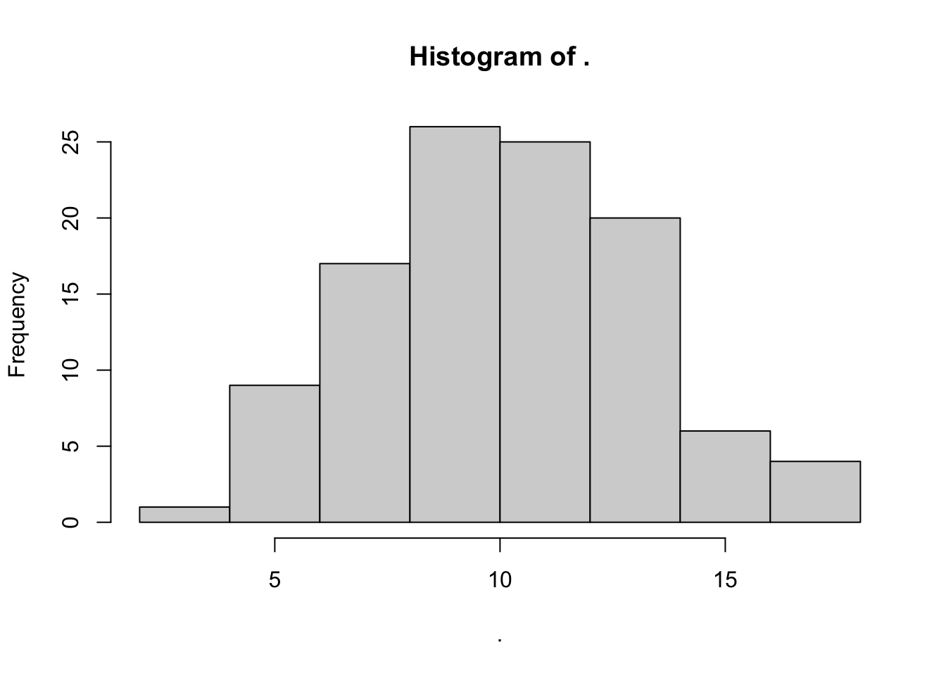
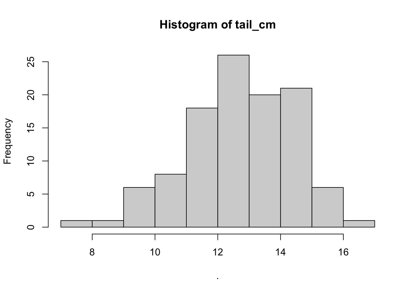
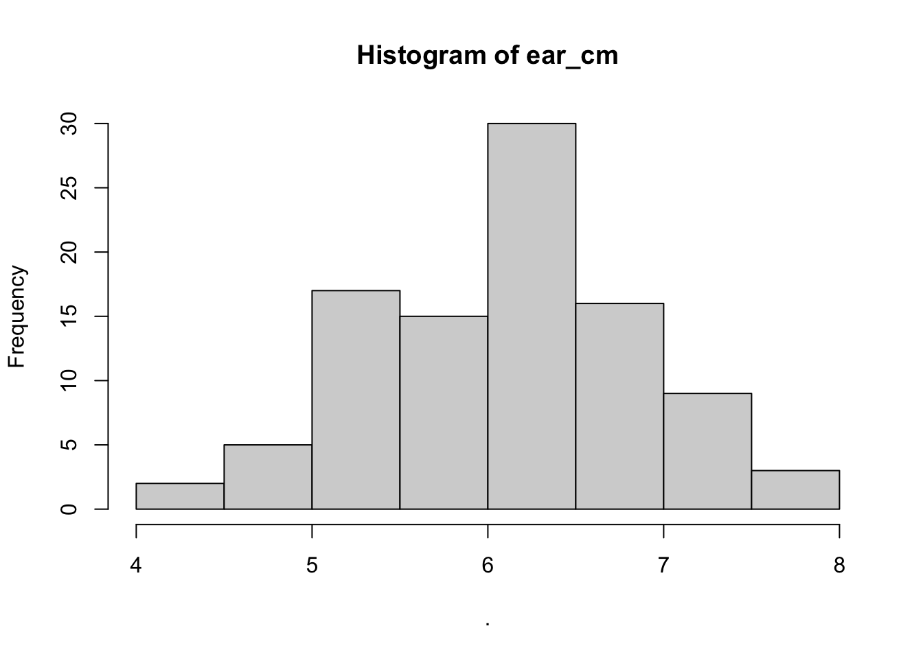
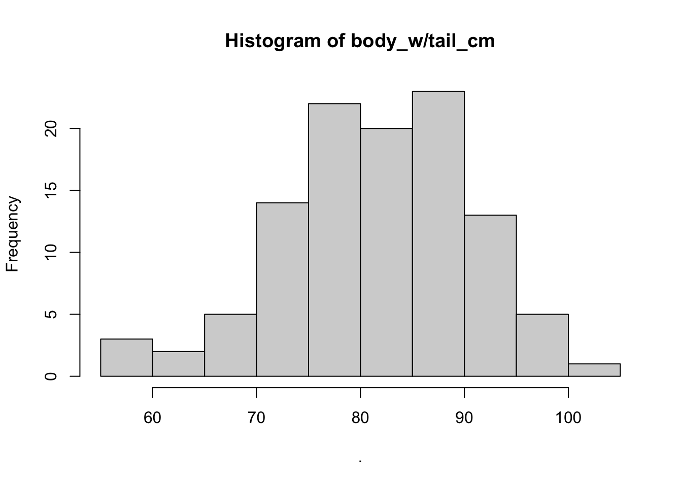
## [1] "histogram"Likely your hiistrograms print without the variable name in the title, which we probably want to know what we are looking at
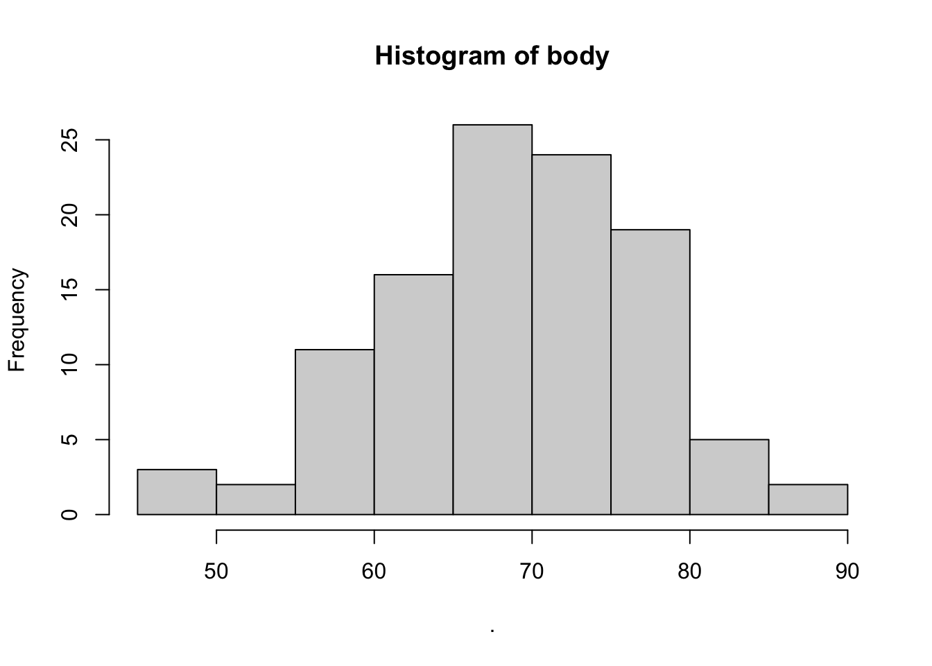
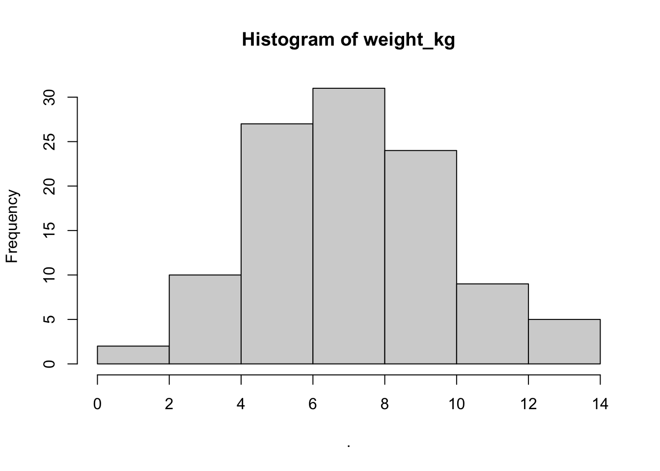
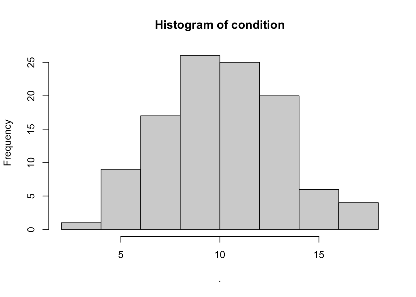
We can accomplish this with imap
First figure out how you would add a main title to a single plot
 Once you’ve done that try adapting this for purrr
bobcat_data$necropsy %>%

  # select only numeric vars
  select(is.numeric) %>%

  # apply purrr::map
  imap(~.x %>%
        #provide histograms
        hist(main = paste('Histogram of', .y))
  )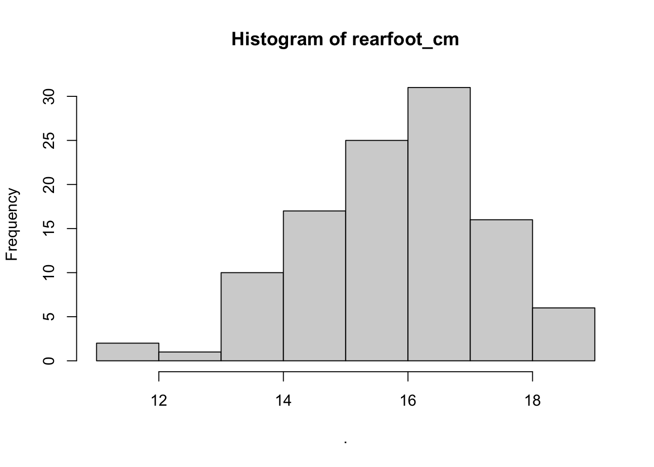
## $rearfoot_cm
## $breaks
## [1] 11 12 13 14 15 16 17 18 19
##
## $counts
## [1]  2  1 10 17 25 31 16  6
##
## $density
## [1] 0.018518519 0.009259259 0.092592593 0.157407407 0.231481481 0.287037037
## [7] 0.148148148 0.055555556
##
## $mids
## [1] 11.5 12.5 13.5 14.5 15.5 16.5 17.5 18.5
##
## $xname
## [1] "."
##
## $equidist
## [1] TRUE
##
## attr(,"class")
## [1] "histogram"
##
## $tail_cm
## $breaks
##  [1]  7  8  9 10 11 12 13 14 15 16 17
##
## $counts
##  [1]  1  1  6  8 18 26 20 21  6  1
##
## $density
##  [1] 0.009259259 0.009259259 0.055555556 0.074074074 0.166666667 0.240740741
##  [7] 0.185185185 0.194444444 0.055555556 0.009259259
##
## $mids
##  [1]  7.5  8.5  9.5 10.5 11.5 12.5 13.5 14.5 15.5 16.5
##
## $xname
## [1] "."
##
## $equidist
## [1] TRUE
##
## attr(,"class")
## [1] "histogram"
##
## $ear_cm
## $breaks
## [1] 4.0 4.5 5.0 5.5 6.0 6.5 7.0 7.5 8.0
##
## $counts
## [1]  2  5 17 15 30 16  9  3
##
## $density
## [1] 0.04123711 0.10309278 0.35051546 0.30927835 0.61855670 0.32989691 0.18556701
## [8] 0.06185567
##
## $mids
## [1] 4.25 4.75 5.25 5.75 6.25 6.75 7.25 7.75
##
## $xname
## [1] "."
##
## $equidist
## [1] TRUE
##
## attr(,"class")
## [1] "histogram"
##
## $`body_w/tail_cm`
## $breaks
##  [1]  55  60  65  70  75  80  85  90  95 100 105
##
## $counts
##  [1]  3  2  5 14 22 20 23 13  5  1
##
## $density
##  [1] 0.005555556 0.003703704 0.009259259 0.025925926 0.040740741 0.037037037
##  [7] 0.042592593 0.024074074 0.009259259 0.001851852
##
## $mids
##  [1]  57.5  62.5  67.5  72.5  77.5  82.5  87.5  92.5  97.5 102.5
##
## $xname
## [1] "."
##
## $equidist
## [1] TRUE
##
## attr(,"class")
## [1] "histogram"
##
## $body
## $breaks
##  [1] 45 50 55 60 65 70 75 80 85 90
##
## $counts
## [1]  3  2 11 16 26 24 19  5  2
##
## $density
## [1] 0.005555556 0.003703704 0.020370370 0.029629630 0.048148148 0.044444444
## [7] 0.035185185 0.009259259 0.003703704
##
## $mids
## [1] 47.5 52.5 57.5 62.5 67.5 72.5 77.5 82.5 87.5
##
## $xname
## [1] "."
##
## $equidist
## [1] TRUE
##
## attr(,"class")
## [1] "histogram"
##
## $weight_kg
## $breaks
## [1]  0  2  4  6  8 10 12 14
##
## $counts
## [1]  2 10 27 31 24  9  5
##
## $density
## [1] 0.009259259 0.046296296 0.125000000 0.143518519 0.111111111 0.041666667
## [7] 0.023148148
##
## $mids
## [1]  1  3  5  7  9 11 13
##
## $xname
## [1] "."
##
## $equidist
## [1] TRUE
##
## attr(,"class")
## [1] "histogram"
##
## $condition
## $breaks
## [1]  2  4  6  8 10 12 14 16 18
##
## $counts
## [1]  1  9 17 26 25 20  6  4
##
## $density
## [1] 0.00462963 0.04166667 0.07870370 0.12037037 0.11574074 0.09259259 0.02777778
## [8] 0.01851852
##
## $mids
## [1]  3  5  7  9 11 13 15 17
##
## $xname
## [1] "."
##
## $equidist
## [1] TRUE
##
## attr(,"class")
## [1] "histogram"
Purrr Map_dfr and map_dfc
Purrr also has a handy function to row-bind and column-bind data when you read it in. This is particularly useful when working with large data sets or data collected over several years.
For example if I had two years of bobcat necropsy data that were entered and saved as separate csv files, I could read them each in individually and then rowbind them together and save this new data frame to my environment to work with later as I’ve done below
# read 2019 data
bobcat_necropsy_2019 <- read_csv('data/raw/sample_bobcat_necropsy_data_2019.csv')
## Rows: 67 Columns: 22
## ── Column specification ────────────────────────────────────────────────────────
## Delimiter: ","
## chr (18): Bobcat_ID#, NecropsyDate, Dissector, County, Township, CollectionD...
## dbl (4): Necropsy, Month, Coordinates_N, Coordinates_W
##
## ℹ Use `spec()` to retrieve the full column specification for this data.
## ℹ Specify the column types or set `show_col_types = FALSE` to quiet this message.# read 2020 data
bobcat_necropsy_2020 <- read_csv('data/raw/sample_bobcat_necropsy_data_2020.csv')## Rows: 44 Columns: 22
## ── Column specification ────────────────────────────────────────────────────────
## Delimiter: ","
## chr (12): Bobcat_ID#, NecropsyDate, Dissector, County, Township, CollectionD...
## dbl (10): Necropsy, Month, Coordinates_N, Coordinates_W, RearFoot_cm, Tail_c...
##
## ℹ Use `spec()` to retrieve the full column specification for this data.
## ℹ Specify the column types or set `show_col_types = FALSE` to quiet this message.bobcat_necropsy_rbind <- rbind(bobcat_necropsy_2019,
bobcat_necropsy_2020)
head(bobcat_necropsy_rbind)## # A tibble: 6 × 22
## `Bobcat_ID#` Necropsy NecropsyDate Dissector County Township CollectionDate
## <chr> <dbl> <chr> <chr> <chr> <chr> <chr>
## 1 5/18/01 1 3/6/19 SP,_MD Athens Dover 12/30/18
## 2 5/18/02 2 3/9/19 SP_MD_CH Athens Canaan 12/14/18
## 3 58-18-03 3 3/10/19 MD_CH Morgan Hower 12/7/18
## 4 64-19-04 4 3/13/19 MD_CH_HK Perry Reading 2/10/19
## 5 34-15-05 5 3/23/19 MD_CH_JG Harrison Monroe 1/11/15
## 6 71-19-06 6 3/24/19 MD_CH Ross Jefferson 3/7/19
## # ℹ 15 more variables: Month <dbl>, Coordinates_N <dbl>, Coordinates_W <dbl>,
## # ApproxAge <chr>, Age <chr>, Sex <chr>, Fecundity_Females <chr>,
## # RearFoot_cm <chr>, Tail_cm <chr>, Ear_cm <chr>, `Body_w/Tail_cm` <chr>,
## # Body <chr>, Weight_kg <chr>, Condition <chr>, Notes <chr>As we can see by looking at the objects in our environment or viewing the data this indeed joined the 2019 data with 2020. But there is a much faster way, especially if you have lots of data files.
Here we use the map_dfr() function in Purrr to
simultaneously rbind our data frames when we read them in. This code
mimics how you would read in multiple data frames into a list except the
function will automatically try to rowbind them instead.
For this to work the columns in the data frame must have the same column type (e.g., character, number, factor etc.) So I’ve also added code to specify how to read in the various columns otherwise we will get an error message.
bobcat_data_dfr <- file.path('data/raw',

                             # provide the names of each data frame
                             c('sample_bobcat_necropsy_data_2019.csv',
                               'sample_bobcat_necropsy_data_2020.csv')) %>%

  # use purrr::map to read in all data at once and rowbind them
  map_dfr(~.x %>%
            read_csv(.,

                     col_types = cols(RearFoot_cm = col_number(),
                                      Tail_cm = col_number(),
                                      Ear_cm = col_number(),
                                      'Body_w/Tail_cm' = col_number(),
                                      Body = col_number(),
                                      Weight_kg = col_number(),
                                      Condition = col_number(),
                                      .default = col_factor())))
## Warning: One or more parsing issues, call `problems()` on your data frame for details,
## e.g.:
## dat <- vroom(...)
## problems(dat)
## One or more parsing issues, call `problems()` on your data frame for details,
## e.g.:
## dat <- vroom(...)
## problems(dat)Now instead of individual data frames or a list object that we have to rbind, in one chunk of code we’ve read in the data and rbdin it so we have a single data frame to work with!
If you have several data files that you want to join via column-bind
you can also use map_dfc() with similar coding as above to
join data frames in this way. But be careful, this function
assumes that the rows in each file are in the same order and nothing is
missing or mismatched, so you can easily get errors if that isn’t the
case. The join functions we covered earlier are a much
safer option because you can specify a ‘key’ to ensure the rows are
matched up properly, but it does take more coding.
We’ve only barely scratched the surface of what Purrr can do, but given our limited time that is where we will end. Just remember anytime you find yourself repeating the same operations for multiple objects of the same type you may want to consider using Purrr instead to reduce repetition in your code.