Assignment 4
GLMs
Due Tuesday February 25th @11:59pm
Submission
Submit you R script as a .R (or .Rmd if using markdown) file to Brightspace.
Please make sure your submission includes your name and the assignment number in the filename
Grading
You should always be following best coding practices (see Intro to R module 1) but especially for assingment submissions.
To receive full credit for each assignment
- Please make sure each problem has its own header so that I can easily navigate to your answers
- Ensure you have comments that explain what you are doing
- Long code chunks should be broken up with spaces and comments to
explain what is happening at each step
- Object names should be lowercase and short but descriptive enough
that they aren’t confused with other objects (For example data1 and
data2 are not good names for dataframes you are working with)
- Just because your code runs doesn’t mean it did what you think it did, always check your data/objects to ensure any functions were performed correctly (there are several ways to do this)
Before you begin
Download data
Make sure you have the Bear glm example raw data (pagube_2008_2016_spatial.csv) downloaded to the data/raw folder.
Readme
Open the README file for this data-set which is associated with Pop et al., 2023 and included in the full (GitHub repository)[https://github.com/marissadyck/Brown_bear_predation_RO] and read about the variables in the pagube_2008_2016_spatial.csv.
Make sure you understand what all the variables are and specifically which could be independent (explanatory) and dependent (response) variables. HINT: there is more than one possible response variable
1 Data import
- First read in the data as a tibble and save it to the environment
with a descriptive and tidy name of your choice
- In the same code chunk as you read the data in, set the column names
to lowercase
- Also in that code chunk, specify how the variables should be read in
(e.g. factor, numeric, etc.)
- Explore the data and make sure things read in properly, make any changes if necessary
bear_damage <- read_csv('data/raw/pagube_2008_2016_spatial.csv',

                        col_types = cols(Damage = col_factor(),
                                         Year = col_factor(),
                                         Month = col_factor(),
                                         Targetspp = col_factor(),
                                         Landcover_code = col_factor(),
                                         .default = col_number())) %>%

  rename_with(tolower)

str(bear_damage)
## spc_tbl_ [3,024 × 24] (S3: spec_tbl_df/tbl_df/tbl/data.frame)
## $ damage : Factor w/ 2 levels "0","1": 1 1 1 1 1 1 2 1 1 2 ...
## $ year : Factor w/ 9 levels "2016","2009",..: 1 2 2 3 4 2 3 4 2 5 ...
## $ month : Factor w/ 12 levels "0","7","9","8",..: 1 1 1 1 1 1 2 1 1 3 ...
## $ targetspp : Factor w/ 3 levels "alte","ovine",..: NA NA NA NA NA NA 1 NA NA 2 ...
## $ point_x : num [1:3024] 489008 491321 491398 491758 492628 ...
## $ point_y : num [1:3024] 532778 542207 538028 536946 533069 ...
## $ bear_abund : num [1:3024] 0 0 26 26 0 26 26 26 26 26 ...
## $ landcover_code : Factor w/ 15 levels "311","112","231",..: 1 1 1 1 1 1 2 3 4 5 ...
## $ altitude : num [1:3024] 549 596 506 485 530 551 437 527 467 561 ...
## $ human_population: num [1:3024] 0 0 54 32 0 0 229 0 0 0 ...
## $ dist_to_forest : num [1:3024] 0 0 0 0 0 ...
## $ dist_to_town : num [1:3024] 1558 2281.6 387.8 60.6 2076.3 ...
## $ livestock_killed: num [1:3024] 0 0 0 0 0 1 1 0 1 1 ...
## $ shannondivindex : num [1:3024] 1.083 0.692 0.908 1.555 0.81 ...
## $ prop_arable : num [1:3024] 0 0 0 14.1 4.7 ...
## $ prop_orchards : num [1:3024] 0 0 0 0 0 0 0 0 0 0 ...
## $ prop_pasture : num [1:3024] 25.2 20.2 42.7 25.4 70.1 ...
## $ prop_ag_mosaic : num [1:3024] 0 0 0 0 0 ...
## $ prop_seminatural: num [1:3024] 9.427 1.668 0.166 22.149 2.001 ...
## $ prop_deciduous : num [1:3024] 59.4 75.7 50.6 27.4 23.2 ...
## $ prop_coniferous : num [1:3024] 0 0 0 0 0 0 0 0 0 0 ...
## $ prop_mixedforest: num [1:3024] 0 0 0 0 0 0 0 0 0 0 ...
## $ prop_grassland : num [1:3024] 0 2.4 0.26 0 0 ...
## $ prop_for_regen : num [1:3024] 4.17 0 0 0 0 ...
## - attr(*, "spec")=
## .. cols(
## .. .default = col_number(),
## .. Damage = col_factor(levels = NULL, ordered = FALSE, include_na = FALSE),
## .. Year = col_factor(levels = NULL, ordered = FALSE, include_na = FALSE),
## .. Month = col_factor(levels = NULL, ordered = FALSE, include_na = FALSE),
## .. Targetspp = col_factor(levels = NULL, ordered = FALSE, include_na = FALSE),
## .. POINT_X = col_number(),
## .. POINT_Y = col_number(),
## .. Bear_abund = col_number(),
## .. Landcover_code = col_factor(levels = NULL, ordered = FALSE, include_na = FALSE),
## .. Altitude = col_number(),
## .. Human_population = col_number(),
## .. Dist_to_forest = col_number(),
## .. Dist_to_town = col_number(),
## .. Livestock_killed = col_number(),
## .. ShannonDivIndex = col_number(),
## .. prop_arable = col_number(),
## .. prop_orchards = col_number(),
## .. prop_pasture = col_number(),
## .. prop_ag_mosaic = col_number(),
## .. prop_seminatural = col_number(),
## .. prop_deciduous = col_number(),
## .. prop_coniferous = col_number(),
## .. prop_mixedforest = col_number(),
## .. prop_grassland = col_number(),
## .. prop_for_regen = col_number()
## .. )
## - attr(*, "problems")=<externalptr>2 Data cleaning
This data has already been cleaned and checked for errors, but to give you some practice with data checking and cleaning I will have you complete the following steps:
- Check that there isn’t any data for years outside the study
specifications, if there are remove those observations
- Check that all entries appear coded correctly for month, if any are
not remove those observations (0s are okay as these are associated with
pseudo-absences)
- create a new variable (with an informative and tidy name of your
choice) that sums all the proportional habitat type observations
(e.g. prop_arable - prop_for_regen) and check that they all sum to 100,
if they don’t filter out the observations that don’t sum to 100 and
assign this data as a new object to the environment with an informative
and tidy name of your choice
- also ensure that this new data set is filtered to only observations where 10 or fewer livestock were killed in an event
- ensure ALL original and new columns are present in this new data set
- when you are done, remove the old data set from the environment, you will use this new cleaned one for future analyses
# check that year is correct
summary(bear_damage$year)
## 2016 2009 2014 2012 2013 2011 2010 2015 2008
## 348 408 396 620 392 160 140 324 236# check that month is correct
summary(bear_damage$month)## 0 7 9 8 5 10 6 4 3 11 12 2
## 2268 139 160 155 84 50 105 27 8 20 7 1# create new data with prop_check column and filter out observations that don't sum to 100
bear_damage_tidy <- bear_damage %>%
mutate(prop_check = rowSums(across(contains('prop')))) %>%
# filter to 100 and only livestock events with 10 or fewer animals
filter(prop_check == 100 &
livestock_killed <= 10)
# check data
summary(bear_damage_tidy)## damage year month targetspp point_x
## 0:922 2012 :245 0 :922 alte : 16 Min. :491321
## 1:198 2013 :160 9 : 42 ovine : 39 1st Qu.:547710
## 2014 :142 6 : 38 bovine:143 Median :569859
## 2015 :136 8 : 34 NA's :922 Mean :575292
## 2009 :132 7 : 31 3rd Qu.:603439
## 2016 :122 5 : 21 Max. :658416
## (Other):183 (Other): 32
## point_y bear_abund landcover_code altitude
## Min. :447121 Min. : 0.00 311 :261 Min. : 255.0
## 1st Qu.:489899 1st Qu.:19.00 312 :254 1st Qu.: 697.0
## Median :519150 Median :31.00 313 :159 Median : 915.0
## Mean :524433 Mean :30.24 321 :135 Mean : 917.8
## 3rd Qu.:552545 3rd Qu.:42.00 231 :129 3rd Qu.:1124.0
## Max. :628579 Max. :77.00 211 : 80 Max. :1707.0
## (Other):102
## human_population dist_to_forest dist_to_town livestock_killed
## Min. : 0.000 Min. : 0.00 Min. : 0 Min. :0.0000
## 1st Qu.: 0.000 1st Qu.: 0.00 1st Qu.: 1790 1st Qu.:0.0000
## Median : 0.000 Median : 0.00 Median : 2941 Median :0.0000
## Mean : 2.546 Mean : 253.24 Mean : 3561 Mean :0.5634
## 3rd Qu.: 0.000 3rd Qu.: 87.58 3rd Qu.: 4770 3rd Qu.:1.0000
## Max. :369.000 Max. :7073.95 Max. :13140 Max. :7.0000
##
## shannondivindex prop_arable prop_orchards prop_pasture
## Min. :0.0000 Min. : 0.000 Min. :0 Min. : 0.00
## 1st Qu.:0.5107 1st Qu.: 0.000 1st Qu.:0 1st Qu.: 0.00
## Median :0.7850 Median : 0.000 Median :0 Median : 0.00
## Mean :0.7633 Mean : 7.002 Mean :0 Mean : 8.88
## 3rd Qu.:1.0451 3rd Qu.: 0.000 3rd Qu.:0 3rd Qu.:11.23
## Max. :1.8951 Max. :100.000 Max. :0 Max. :96.11
##
## prop_ag_mosaic prop_seminatural prop_deciduous prop_coniferous
## Min. : 0.0000 Min. : 0.000 Min. : 0.00 Min. : 0.000
## 1st Qu.: 0.0000 1st Qu.: 0.000 1st Qu.: 0.00 1st Qu.: 0.000
## Median : 0.0000 Median : 0.000 Median : 3.13 Median : 6.774
## Mean : 0.8042 Mean : 1.753 Mean : 27.40 Mean : 24.417
## 3rd Qu.: 0.0000 3rd Qu.: 0.000 3rd Qu.: 56.59 3rd Qu.: 45.989
## Max. :42.9740 Max. :44.391 Max. :100.00 Max. :100.000
##
## prop_mixedforest prop_grassland prop_for_regen prop_check
## Min. : 0.00 Min. : 0.000 Min. : 0.000 Min. :100
## 1st Qu.: 0.00 1st Qu.: 0.000 1st Qu.: 0.000 1st Qu.:100
## Median : 0.00 Median : 0.000 Median : 0.000 Median :100
## Mean : 15.26 Mean : 8.732 Mean : 5.758 Mean :100
## 3rd Qu.: 22.11 3rd Qu.:13.614 3rd Qu.: 8.162 3rd Qu.:100
## Max. :100.00 Max. :86.540 Max. :61.234 Max. :100
## # remove old data
rm(bear_damage)3 Summary statistics
Using your new data set, please calculate some summary statistics to report
- Total number of events AND total number of livestock killed by brown
bears across the entire study
- Total number of events of your response variable per livestock type,
year, and month provide comments that highlight which type, year,
and month had the most and least number of events
- Number of events of your response variable per livestock type for each year provide comments that highlight which year had the most and least number of events for each livestock type
# total number of events & livestock killed
bear_damage_tidy %>%

  # ensure to only count events of damage
  filter(damage == '1') %>%

  summarise(n_events = n(),
            total_killed = sum(livestock_killed))
## # A tibble: 1 × 2
## n_events total_killed
## <int> <dbl>
## 1 198 470# damage per species
bear_damage_tidy %>%
# ensure to only count events of damage
filter(damage == '1') %>%
# group by targetspp to get summaries for each species and year
group_by(targetspp) %>%
summarise(n = n())## # A tibble: 3 × 2
## targetspp n
## <fct> <int>
## 1 alte 16
## 2 ovine 39
## 3 bovine 143# bovine highest, alte lowest
# damage per year
bear_damage_tidy %>%
# ensure to only count events of damage
filter(damage == '1') %>%
# group by targetspp to get summaries for each species and year
group_by(year) %>%
summarise(n = n()) %>%
arrange(desc(n))## # A tibble: 9 × 2
## year n
## <fct> <int>
## 1 2012 42
## 2 2013 34
## 3 2014 28
## 4 2016 26
## 5 2015 25
## 6 2009 12
## 7 2011 11
## 8 2010 11
## 9 2008 9# 2012 had highest number of events and 2008 had lowest number of events
# damage per month
bear_damage_tidy %>%
# ensure to only count events of damage
filter(damage == '1') %>%
# group by targetspp to get summaries for each species and year
group_by(month) %>%
summarise(n = n()) %>%
arrange(desc(n))## # A tibble: 10 × 2
## month n
## <fct> <int>
## 1 9 42
## 2 6 38
## 3 8 34
## 4 7 31
## 5 5 21
## 6 10 14
## 7 4 12
## 8 11 4
## 9 3 1
## 10 2 1# september had the highest number of events and Dec/Jan had lowest with 0
# damage per livestock type per year
bear_damage_tidy %>%
# ensure to only count events of damage
filter(damage == '1') %>%
# group by targetspp to get summaries for each species and year
group_by(targetspp, year) %>%
summarise(n = n()) %>%
arrange(desc(n))## `summarise()` has grouped output by 'targetspp'. You can override using the
## `.groups` argument.## # A tibble: 25 × 3
## # Groups: targetspp [3]
## targetspp year n
## <fct> <fct> <int>
## 1 bovine 2012 31
## 2 bovine 2013 30
## 3 bovine 2015 22
## 4 bovine 2014 21
## 5 bovine 2016 18
## 6 bovine 2011 8
## 7 ovine 2016 7
## 8 ovine 2012 7
## 9 ovine 2008 7
## 10 bovine 2010 7
## # ℹ 15 more rows# 4 Identify the response variable
Once your data are cleaned and formatted please identify the response variable for your models (There are two possible response variables)
AND the appropriate distribution for your data You’ll need to provide some kind of code to show you looked at the response variable to choose the distribution
# damage is response variable and the appropriate distribution is binomial

plot(bear_damage_tidy$damage)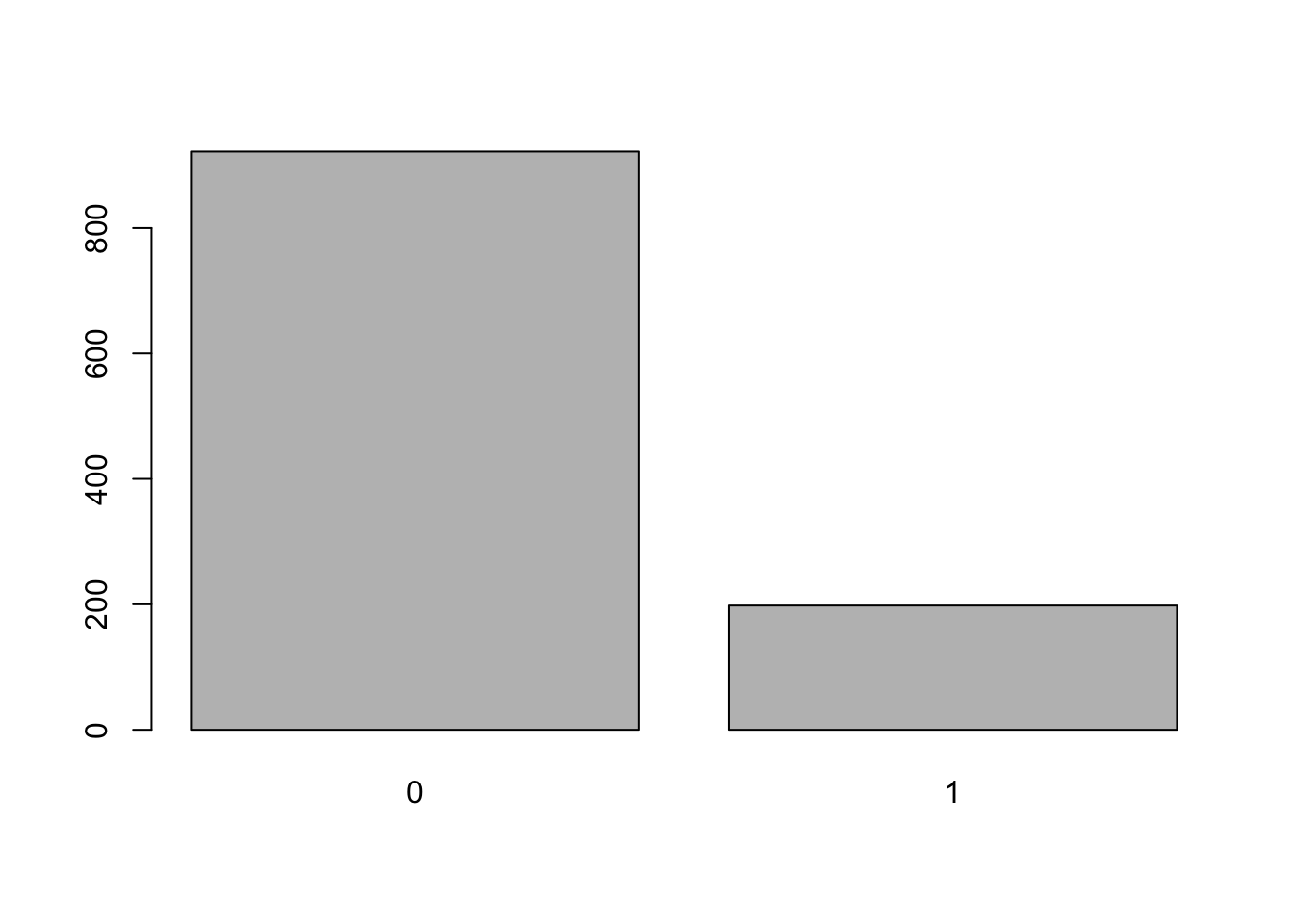
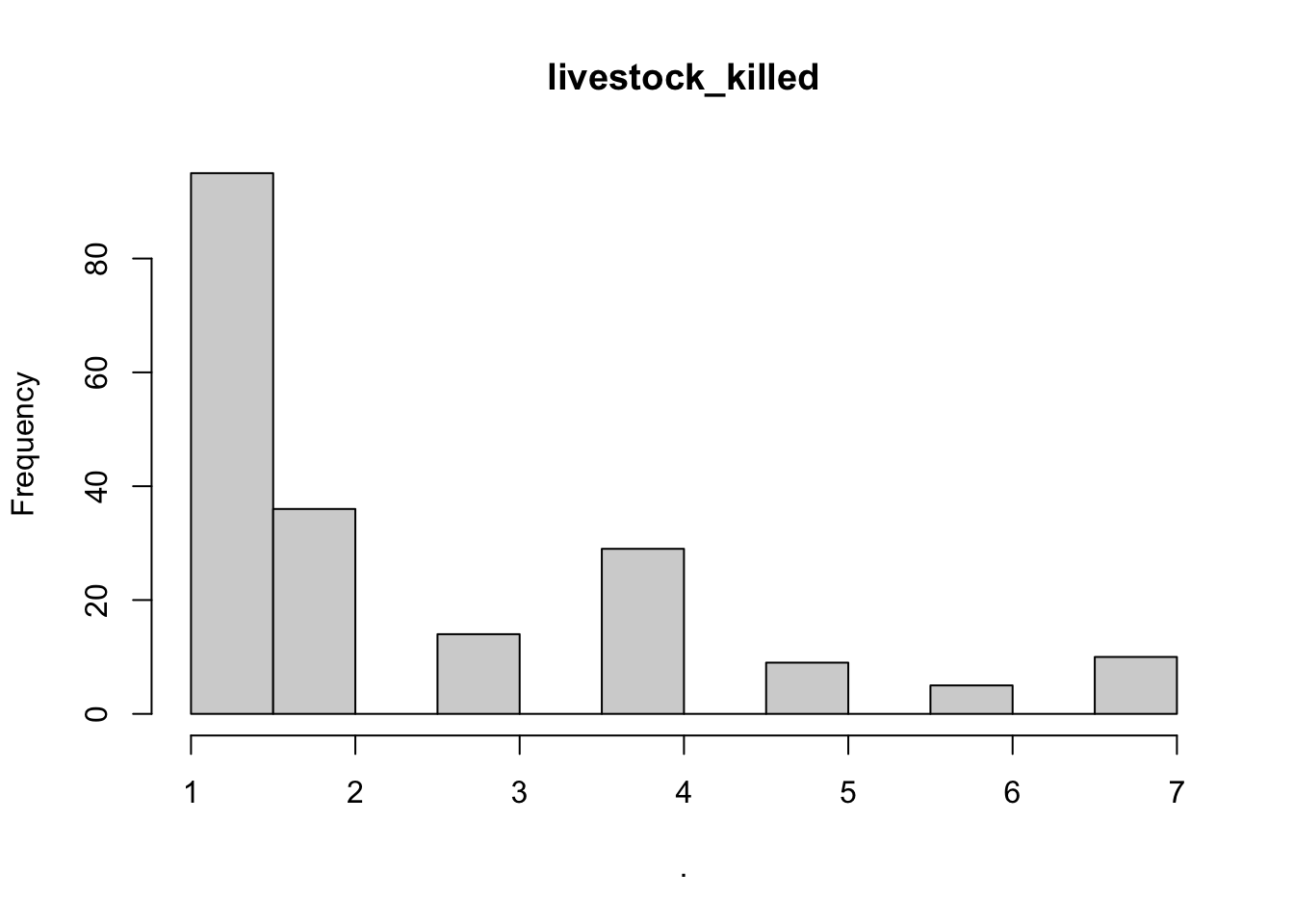
# or livestock killed is response variable which is count data so could be poisson or if highly zero-inflated causes overdispersion then negative binomial
hist(bear_damage_tidy$livestock_killed)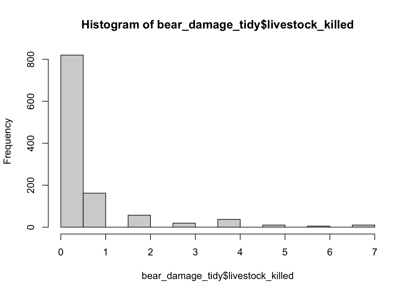
# lots of zeros lets do a quick test for dispersion with a simple glm
test_glm <-
glm(livestock_killed ~ bear_abund,
    data = bear_damage_tidy,
    family = 'poisson')

summary(test_glm)
##
## Call:
## glm(formula = livestock_killed ~ bear_abund, family = "poisson",
## data = bear_damage_tidy)
##
## Deviance Residuals:
## Min 1Q Median 3Q Max
## -1.4672 -1.0886 -0.9689 0.3295 4.8808
##
## Coefficients:
## Estimate Std. Error z value Pr(>|z|)
## (Intercept) -1.047516 0.087835 -11.926 < 2e-16 ***
## bear_abund 0.014560 0.002248 6.477 9.34e-11 ***
## ---
## Signif. codes: 0 '***' 0.001 '**' 0.01 '*' 0.05 '.' 0.1 ' ' 1
##
## (Dispersion parameter for poisson family taken to be 1)
##
## Null deviance: 1958.6 on 1119 degrees of freedom
## Residual deviance: 1916.5 on 1118 degrees of freedom
## AIC: 2662.3
##
## Number of Fisher Scoring iterations: 6# calculate dispersion
1916.5/1118## [1] 1.714222# 1.74 is high so over-dispersed - use negative binomial5 Data exploration
Then complete the data exploration steps below
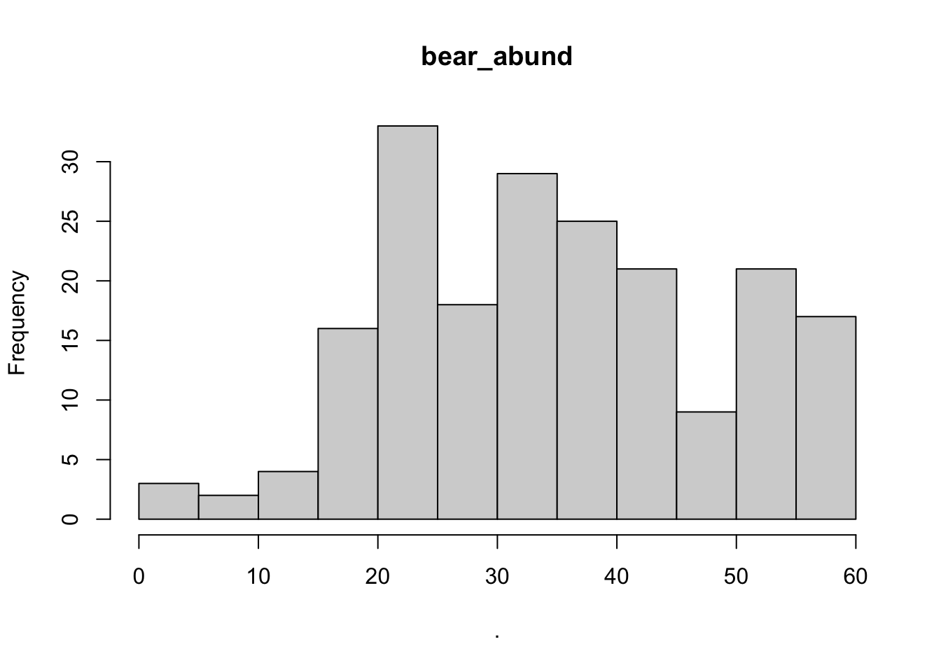
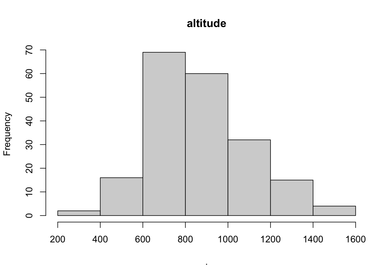
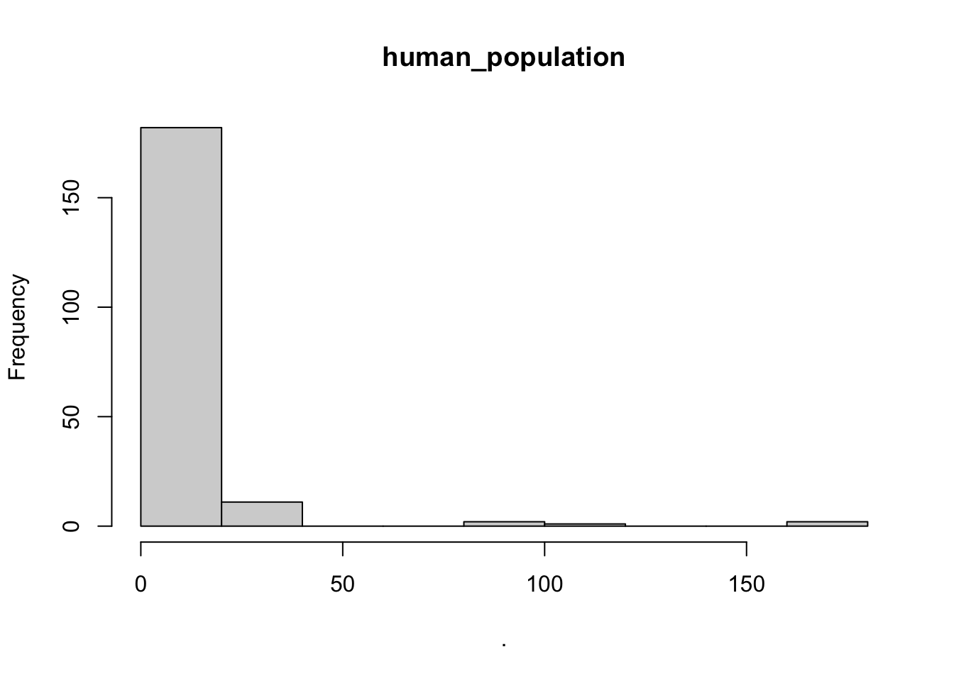
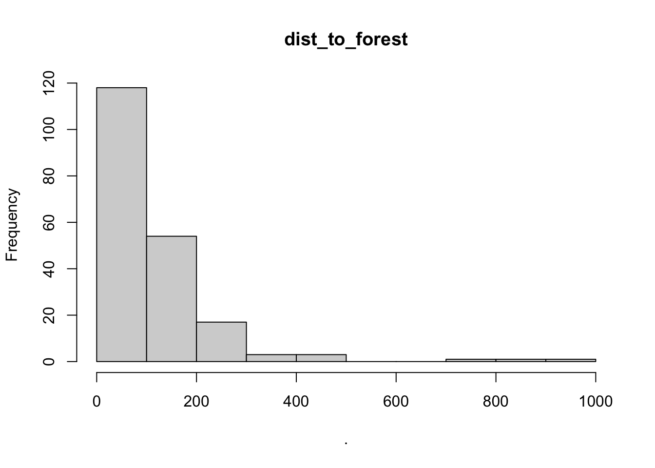
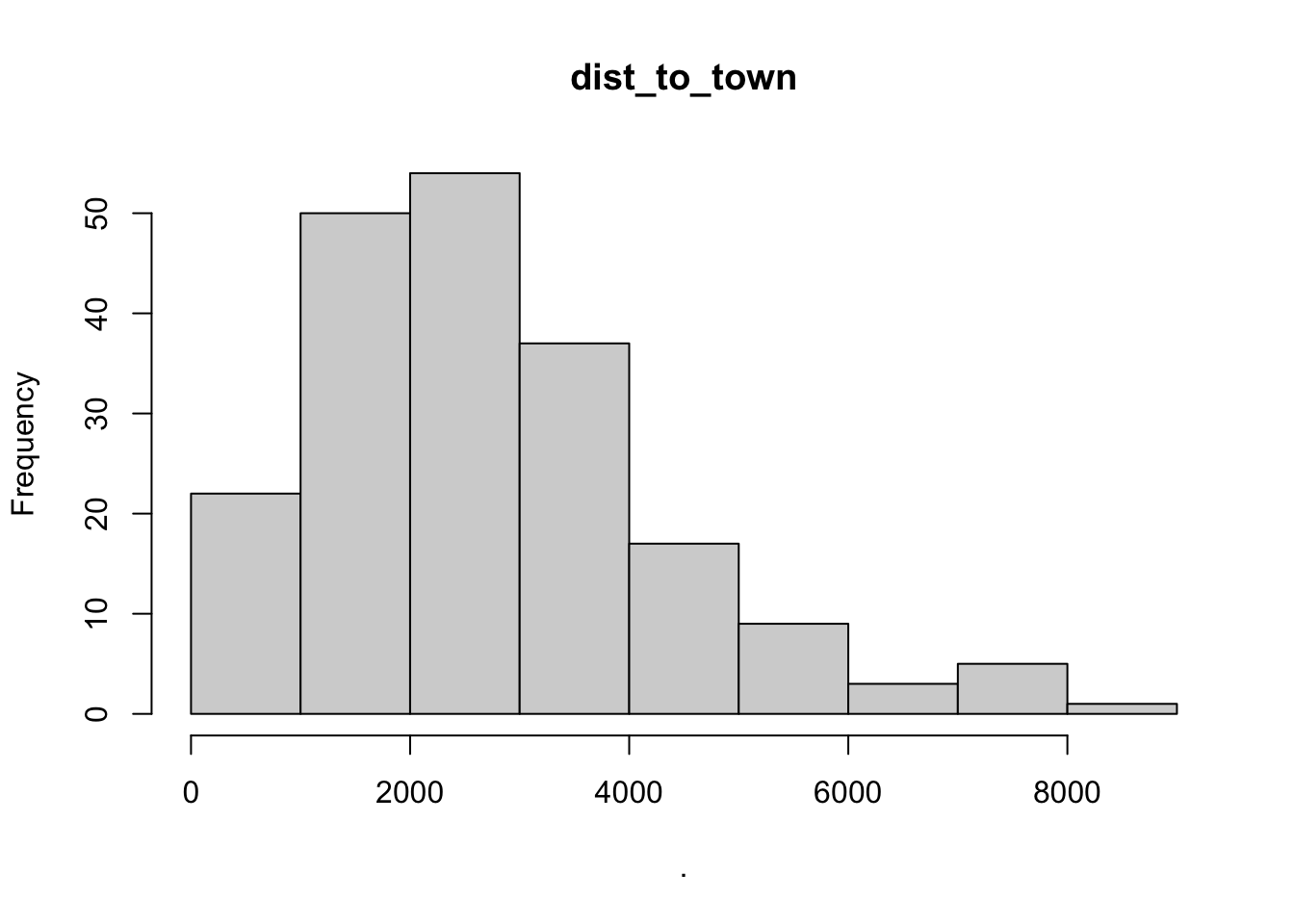
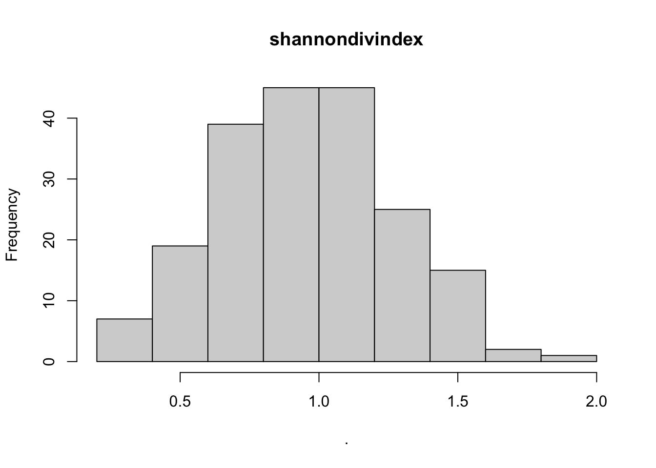
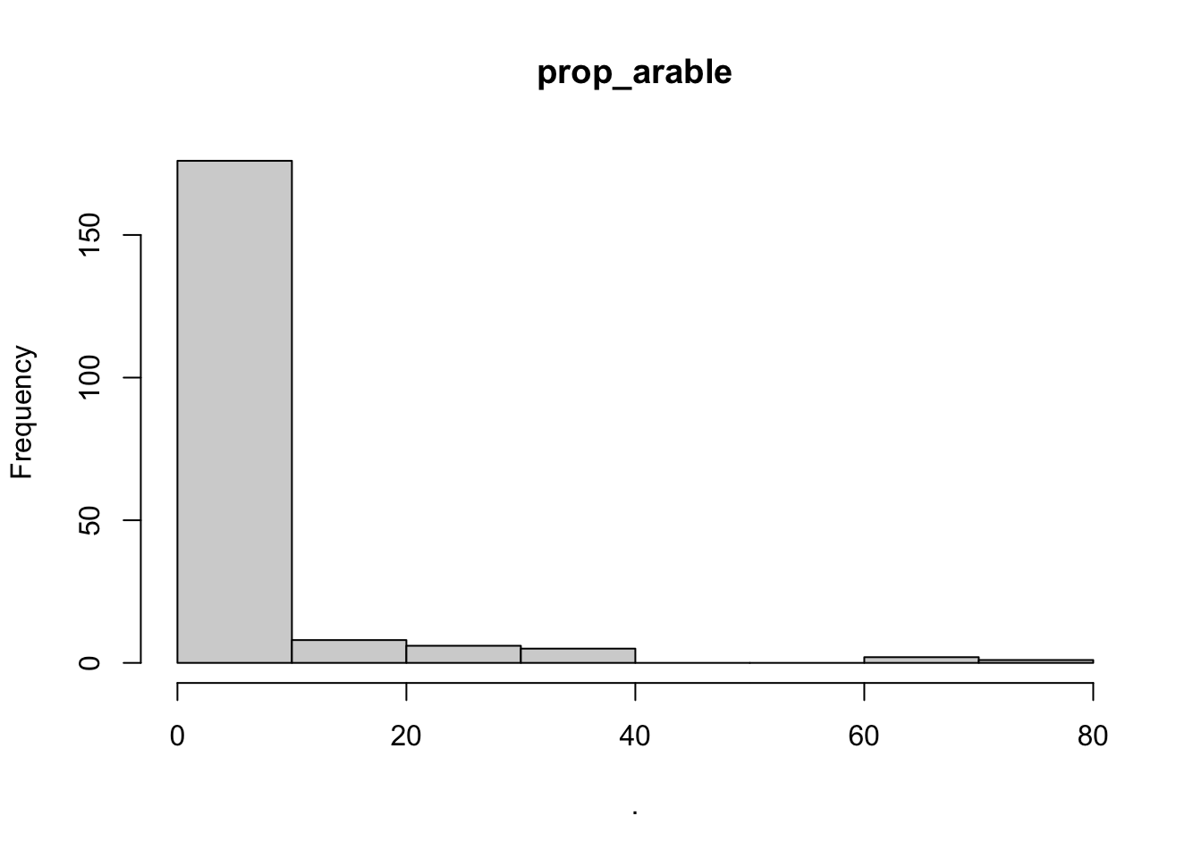
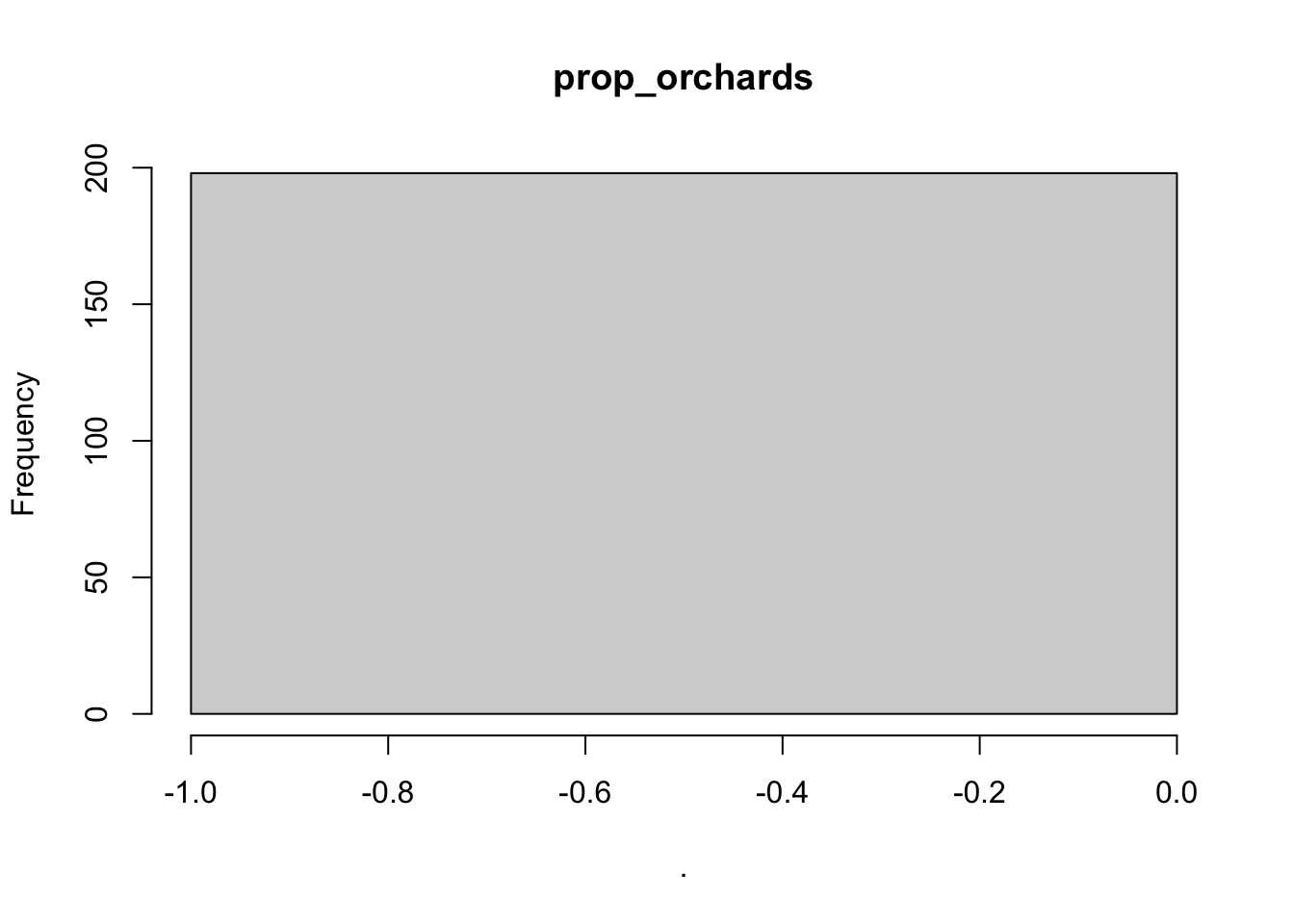
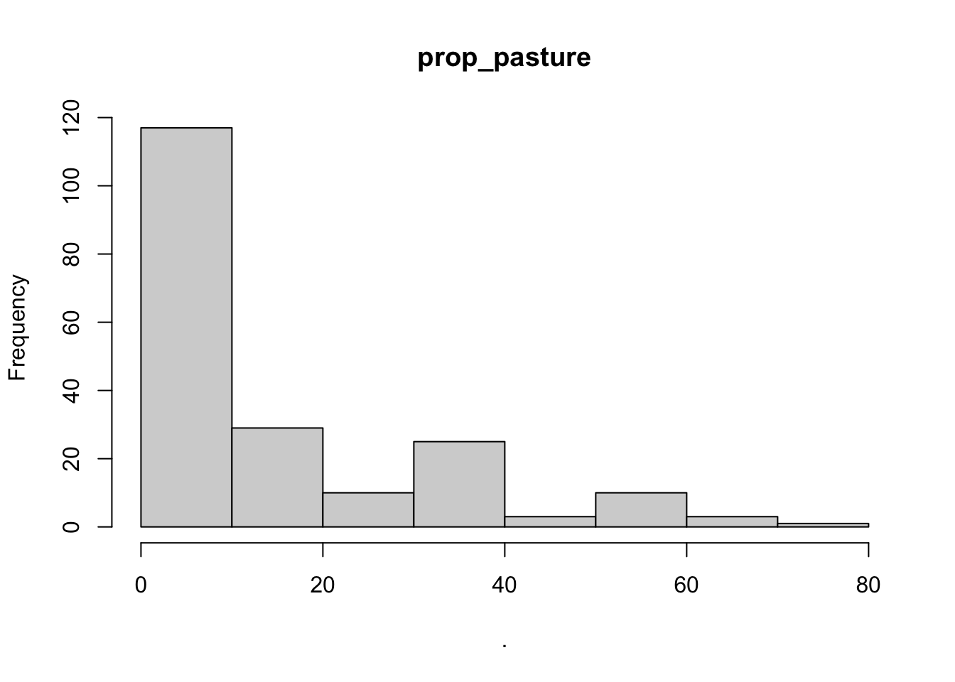
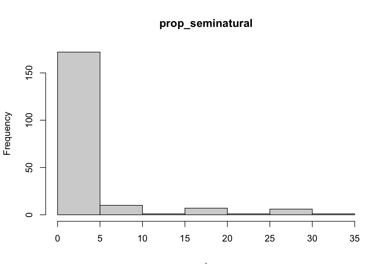
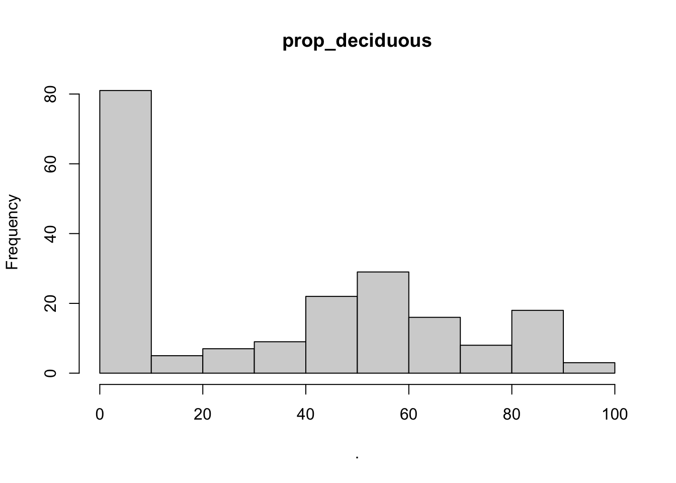
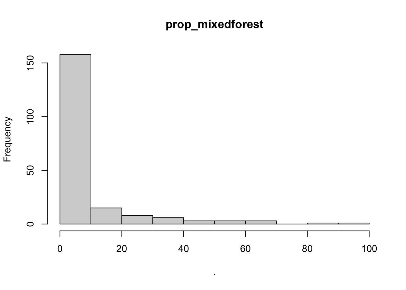
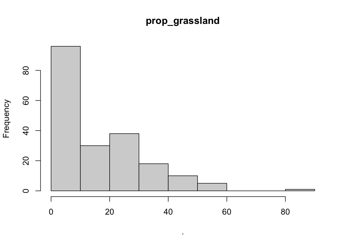
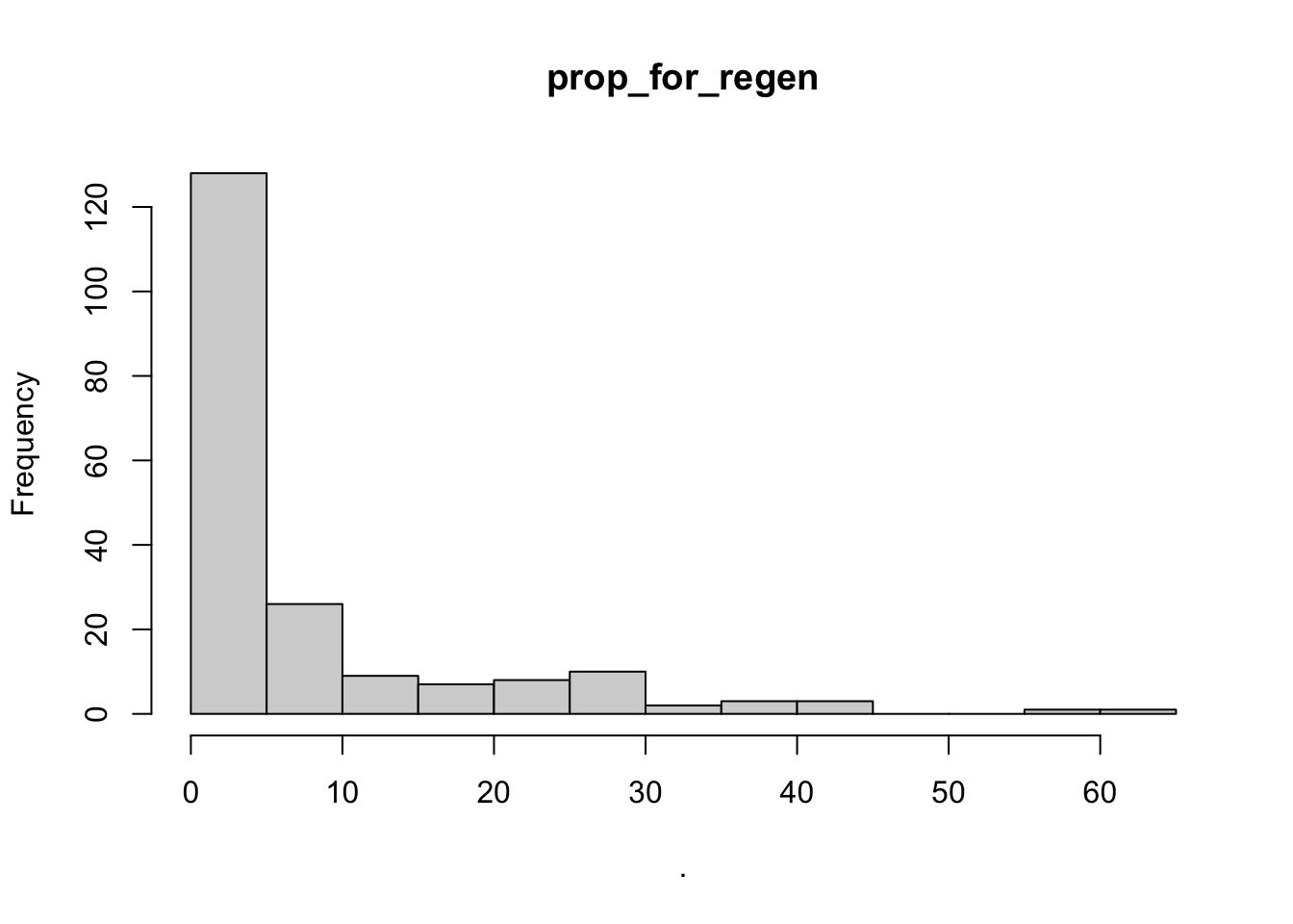
- Generate plots of your potential explanatory variables and determine which are useful (provide annotation of why some are not useful)
- From the selected candidate explanatory variables check for multicolinearity between variables and make note of which variables are highly correlated and the r2 value.
# using purr
bear_damage_tidy %>%

  filter(damage == '1') %>%

  select_if(is.numeric) %>%

  # use imap which will retain both the data (x) and the variable names (y)
  imap(~.x %>%

         # use the hist function on the data from previous pipe
        hist(.,

             # set the main title to y (each variable)
             main = .y))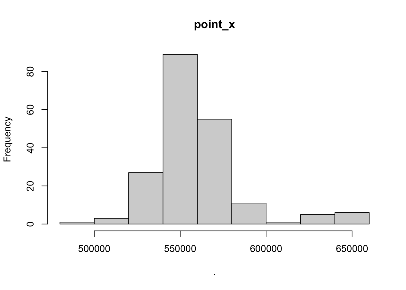
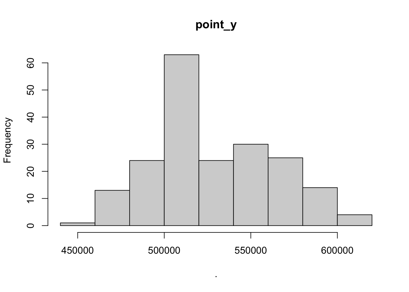


## $point_x
## $breaks
##  [1] 480000 500000 520000 540000 560000 580000 600000 620000 640000 660000
##
## $counts
## [1]  1  3 27 89 55 11  1  5  6
##
## $density
## [1] 2.525253e-07 7.575758e-07 6.818182e-06 2.247475e-05 1.388889e-05
## [6] 2.777778e-06 2.525253e-07 1.262626e-06 1.515152e-06
##
## $mids
## [1] 490000 510000 530000 550000 570000 590000 610000 630000 650000
##
## $xname
## [1] "."
##
## $equidist
## [1] TRUE
##
## attr(,"class")
## [1] "histogram"
##
## $point_y
## $breaks
##  [1] 440000 460000 480000 500000 520000 540000 560000 580000 600000 620000
##
## $counts
## [1]  1 13 24 63 24 30 25 14  4
##
## $density
## [1] 2.525253e-07 3.282828e-06 6.060606e-06 1.590909e-05 6.060606e-06
## [6] 7.575758e-06 6.313131e-06 3.535354e-06 1.010101e-06
##
## $mids
## [1] 450000 470000 490000 510000 530000 550000 570000 590000 610000
##
## $xname
## [1] "."
##
## $equidist
## [1] TRUE
##
## attr(,"class")
## [1] "histogram"
##
## $bear_abund
## $breaks
##  [1]  0  5 10 15 20 25 30 35 40 45 50 55 60
##
## $counts
##  [1]  3  2  4 16 33 18 29 25 21  9 21 17
##
## $density
##  [1] 0.003030303 0.002020202 0.004040404 0.016161616 0.033333333 0.018181818
##  [7] 0.029292929 0.025252525 0.021212121 0.009090909 0.021212121 0.017171717
##
## $mids
##  [1]  2.5  7.5 12.5 17.5 22.5 27.5 32.5 37.5 42.5 47.5 52.5 57.5
##
## $xname
## [1] "."
##
## $equidist
## [1] TRUE
##
## attr(,"class")
## [1] "histogram"
##
## $altitude
## $breaks
## [1]  200  400  600  800 1000 1200 1400 1600
##
## $counts
## [1]  2 16 69 60 32 15  4
##
## $density
## [1] 5.050505e-05 4.040404e-04 1.742424e-03 1.515152e-03 8.080808e-04
## [6] 3.787879e-04 1.010101e-04
##
## $mids
## [1]  300  500  700  900 1100 1300 1500
##
## $xname
## [1] "."
##
## $equidist
## [1] TRUE
##
## attr(,"class")
## [1] "histogram"
##
## $human_population
## $breaks
##  [1]   0  20  40  60  80 100 120 140 160 180
##
## $counts
## [1] 182  11   0   0   2   1   0   0   2
##
## $density
## [1] 0.0459595960 0.0027777778 0.0000000000 0.0000000000 0.0005050505
## [6] 0.0002525253 0.0000000000 0.0000000000 0.0005050505
##
## $mids
## [1]  10  30  50  70  90 110 130 150 170
##
## $xname
## [1] "."
##
## $equidist
## [1] TRUE
##
## attr(,"class")
## [1] "histogram"
##
## $dist_to_forest
## $breaks
##  [1]    0  100  200  300  400  500  600  700  800  900 1000
##
## $counts
##  [1] 118  54  17   3   3   0   0   1   1   1
##
## $density
##  [1] 5.959596e-03 2.727273e-03 8.585859e-04 1.515152e-04 1.515152e-04
##  [6] 0.000000e+00 0.000000e+00 5.050505e-05 5.050505e-05 5.050505e-05
##
## $mids
##  [1]  50 150 250 350 450 550 650 750 850 950
##
## $xname
## [1] "."
##
## $equidist
## [1] TRUE
##
## attr(,"class")
## [1] "histogram"
##
## $dist_to_town
## $breaks
##  [1]    0 1000 2000 3000 4000 5000 6000 7000 8000 9000
##
## $counts
## [1] 22 50 54 37 17  9  3  5  1
##
## $density
## [1] 1.111111e-04 2.525253e-04 2.727273e-04 1.868687e-04 8.585859e-05
## [6] 4.545455e-05 1.515152e-05 2.525253e-05 5.050505e-06
##
## $mids
## [1]  500 1500 2500 3500 4500 5500 6500 7500 8500
##
## $xname
## [1] "."
##
## $equidist
## [1] TRUE
##
## attr(,"class")
## [1] "histogram"
##
## $livestock_killed
## $breaks
##  [1] 1.0 1.5 2.0 2.5 3.0 3.5 4.0 4.5 5.0 5.5 6.0 6.5 7.0
##
## $counts
##  [1] 95 36  0 14  0 29  0  9  0  5  0 10
##
## $density
##  [1] 0.95959596 0.36363636 0.00000000 0.14141414 0.00000000 0.29292929
##  [7] 0.00000000 0.09090909 0.00000000 0.05050505 0.00000000 0.10101010
##
## $mids
##  [1] 1.25 1.75 2.25 2.75 3.25 3.75 4.25 4.75 5.25 5.75 6.25 6.75
##
## $xname
## [1] "."
##
## $equidist
## [1] TRUE
##
## attr(,"class")
## [1] "histogram"
##
## $shannondivindex
## $breaks
##  [1] 0.2 0.4 0.6 0.8 1.0 1.2 1.4 1.6 1.8 2.0
##
## $counts
## [1]  7 19 39 45 45 25 15  2  1
##
## $density
## [1] 0.17676768 0.47979798 0.98484848 1.13636364 1.13636364 0.63131313 0.37878788
## [8] 0.05050505 0.02525253
##
## $mids
## [1] 0.3 0.5 0.7 0.9 1.1 1.3 1.5 1.7 1.9
##
## $xname
## [1] "."
##
## $equidist
## [1] TRUE
##
## attr(,"class")
## [1] "histogram"
##
## $prop_arable
## $breaks
## [1]  0 10 20 30 40 50 60 70 80
##
## $counts
## [1] 176   8   6   5   0   0   2   1
##
## $density
## [1] 0.0888888889 0.0040404040 0.0030303030 0.0025252525 0.0000000000
## [6] 0.0000000000 0.0010101010 0.0005050505
##
## $mids
## [1]  5 15 25 35 45 55 65 75
##
## $xname
## [1] "."
##
## $equidist
## [1] TRUE
##
## attr(,"class")
## [1] "histogram"
##
## $prop_orchards
## $breaks
## [1] -1  0
##
## $counts
## [1] 198
##
## $density
## [1] 1
##
## $mids
## [1] -0.5
##
## $xname
## [1] "."
##
## $equidist
## [1] TRUE
##
## attr(,"class")
## [1] "histogram"
##
## $prop_pasture
## $breaks
## [1]  0 10 20 30 40 50 60 70 80
##
## $counts
## [1] 117  29  10  25   3  10   3   1
##
## $density
## [1] 0.0590909091 0.0146464646 0.0050505051 0.0126262626 0.0015151515
## [6] 0.0050505051 0.0015151515 0.0005050505
##
## $mids
## [1]  5 15 25 35 45 55 65 75
##
## $xname
## [1] "."
##
## $equidist
## [1] TRUE
##
## attr(,"class")
## [1] "histogram"
##
## $prop_ag_mosaic
## $breaks
##  [1]  0  5 10 15 20 25 30 35 40 45
##
## $counts
## [1] 186   5   0   3   0   3   0   0   1
##
## $density
## [1] 0.187878788 0.005050505 0.000000000 0.003030303 0.000000000 0.003030303
## [7] 0.000000000 0.000000000 0.001010101
##
## $mids
## [1]  2.5  7.5 12.5 17.5 22.5 27.5 32.5 37.5 42.5
##
## $xname
## [1] "."
##
## $equidist
## [1] TRUE
##
## attr(,"class")
## [1] "histogram"
##
## $prop_seminatural
## $breaks
## [1]  0  5 10 15 20 25 30 35
##
## $counts
## [1] 172  10   1   7   1   6   1
##
## $density
## [1] 0.173737374 0.010101010 0.001010101 0.007070707 0.001010101 0.006060606
## [7] 0.001010101
##
## $mids
## [1]  2.5  7.5 12.5 17.5 22.5 27.5 32.5
##
## $xname
## [1] "."
##
## $equidist
## [1] TRUE
##
## attr(,"class")
## [1] "histogram"
##
## $prop_deciduous
## $breaks
##  [1]   0  10  20  30  40  50  60  70  80  90 100
##
## $counts
##  [1] 81  5  7  9 22 29 16  8 18  3
##
## $density
##  [1] 0.040909091 0.002525253 0.003535354 0.004545455 0.011111111 0.014646465
##  [7] 0.008080808 0.004040404 0.009090909 0.001515152
##
## $mids
##  [1]  5 15 25 35 45 55 65 75 85 95
##
## $xname
## [1] "."
##
## $equidist
## [1] TRUE
##
## attr(,"class")
## [1] "histogram"
##
## $prop_coniferous
## $breaks
##  [1]  0 10 20 30 40 50 60 70 80 90
##
## $counts
## [1] 118  20  11  10  13  10   8   6   2
##
## $density
## [1] 0.059595960 0.010101010 0.005555556 0.005050505 0.006565657 0.005050505
## [7] 0.004040404 0.003030303 0.001010101
##
## $mids
## [1]  5 15 25 35 45 55 65 75 85
##
## $xname
## [1] "."
##
## $equidist
## [1] TRUE
##
## attr(,"class")
## [1] "histogram"
##
## $prop_mixedforest
## $breaks
##  [1]   0  10  20  30  40  50  60  70  80  90 100
##
## $counts
##  [1] 158  15   8   6   3   3   3   0   1   1
##
## $density
##  [1] 0.0797979798 0.0075757576 0.0040404040 0.0030303030 0.0015151515
##  [6] 0.0015151515 0.0015151515 0.0000000000 0.0005050505 0.0005050505
##
## $mids
##  [1]  5 15 25 35 45 55 65 75 85 95
##
## $xname
## [1] "."
##
## $equidist
## [1] TRUE
##
## attr(,"class")
## [1] "histogram"
##
## $prop_grassland
## $breaks
##  [1]  0 10 20 30 40 50 60 70 80 90
##
## $counts
## [1] 96 30 38 18 10  5  0  0  1
##
## $density
## [1] 0.0484848485 0.0151515152 0.0191919192 0.0090909091 0.0050505051
## [6] 0.0025252525 0.0000000000 0.0000000000 0.0005050505
##
## $mids
## [1]  5 15 25 35 45 55 65 75 85
##
## $xname
## [1] "."
##
## $equidist
## [1] TRUE
##
## attr(,"class")
## [1] "histogram"
##
## $prop_for_regen
## $breaks
##  [1]  0  5 10 15 20 25 30 35 40 45 50 55 60 65
##
## $counts
##  [1] 128  26   9   7   8  10   2   3   3   0   0   1   1
##
## $density
##  [1] 0.129292929 0.026262626 0.009090909 0.007070707 0.008080808 0.010101010
##  [7] 0.002020202 0.003030303 0.003030303 0.000000000 0.000000000 0.001010101
## [13] 0.001010101
##
## $mids
##  [1]  2.5  7.5 12.5 17.5 22.5 27.5 32.5 37.5 42.5 47.5 52.5 57.5 62.5
##
## $xname
## [1] "."
##
## $equidist
## [1] TRUE
##
## attr(,"class")
## [1] "histogram"
##
## $prop_check
## $breaks
## [1]  80 100
##
## $counts
## [1] 198
##
## $density
## [1] 0.05
##
## $mids
## [1] 90
##
## $xname
## [1] "."
##
## $equidist
## [1] TRUE
##
## attr(,"class")
## [1] "histogram"summary(bear_damage_tidy)## damage year month targetspp point_x
## 0:922 2012 :245 0 :922 alte : 16 Min. :491321
## 1:198 2013 :160 9 : 42 ovine : 39 1st Qu.:547710
## 2014 :142 6 : 38 bovine:143 Median :569859
## 2015 :136 8 : 34 NA's :922 Mean :575292
## 2009 :132 7 : 31 3rd Qu.:603439
## 2016 :122 5 : 21 Max. :658416
## (Other):183 (Other): 32
## point_y bear_abund landcover_code altitude
## Min. :447121 Min. : 0.00 311 :261 Min. : 255.0
## 1st Qu.:489899 1st Qu.:19.00 312 :254 1st Qu.: 697.0
## Median :519150 Median :31.00 313 :159 Median : 915.0
## Mean :524433 Mean :30.24 321 :135 Mean : 917.8
## 3rd Qu.:552545 3rd Qu.:42.00 231 :129 3rd Qu.:1124.0
## Max. :628579 Max. :77.00 211 : 80 Max. :1707.0
## (Other):102
## human_population dist_to_forest dist_to_town livestock_killed
## Min. : 0.000 Min. : 0.00 Min. : 0 Min. :0.0000
## 1st Qu.: 0.000 1st Qu.: 0.00 1st Qu.: 1790 1st Qu.:0.0000
## Median : 0.000 Median : 0.00 Median : 2941 Median :0.0000
## Mean : 2.546 Mean : 253.24 Mean : 3561 Mean :0.5634
## 3rd Qu.: 0.000 3rd Qu.: 87.58 3rd Qu.: 4770 3rd Qu.:1.0000
## Max. :369.000 Max. :7073.95 Max. :13140 Max. :7.0000
##
## shannondivindex prop_arable prop_orchards prop_pasture
## Min. :0.0000 Min. : 0.000 Min. :0 Min. : 0.00
## 1st Qu.:0.5107 1st Qu.: 0.000 1st Qu.:0 1st Qu.: 0.00
## Median :0.7850 Median : 0.000 Median :0 Median : 0.00
## Mean :0.7633 Mean : 7.002 Mean :0 Mean : 8.88
## 3rd Qu.:1.0451 3rd Qu.: 0.000 3rd Qu.:0 3rd Qu.:11.23
## Max. :1.8951 Max. :100.000 Max. :0 Max. :96.11
##
## prop_ag_mosaic prop_seminatural prop_deciduous prop_coniferous
## Min. : 0.0000 Min. : 0.000 Min. : 0.00 Min. : 0.000
## 1st Qu.: 0.0000 1st Qu.: 0.000 1st Qu.: 0.00 1st Qu.: 0.000
## Median : 0.0000 Median : 0.000 Median : 3.13 Median : 6.774
## Mean : 0.8042 Mean : 1.753 Mean : 27.40 Mean : 24.417
## 3rd Qu.: 0.0000 3rd Qu.: 0.000 3rd Qu.: 56.59 3rd Qu.: 45.989
## Max. :42.9740 Max. :44.391 Max. :100.00 Max. :100.000
##
## prop_mixedforest prop_grassland prop_for_regen prop_check
## Min. : 0.00 Min. : 0.000 Min. : 0.000 Min. :100
## 1st Qu.: 0.00 1st Qu.: 0.000 1st Qu.: 0.000 1st Qu.:100
## Median : 0.00 Median : 0.000 Median : 0.000 Median :100
## Mean : 15.26 Mean : 8.732 Mean : 5.758 Mean :100
## 3rd Qu.: 22.11 3rd Qu.:13.614 3rd Qu.: 8.162 3rd Qu.:100
## Max. :100.00 Max. :86.540 Max. :61.234 Max. :100
## plot(bear_damage_tidy$landcover_code)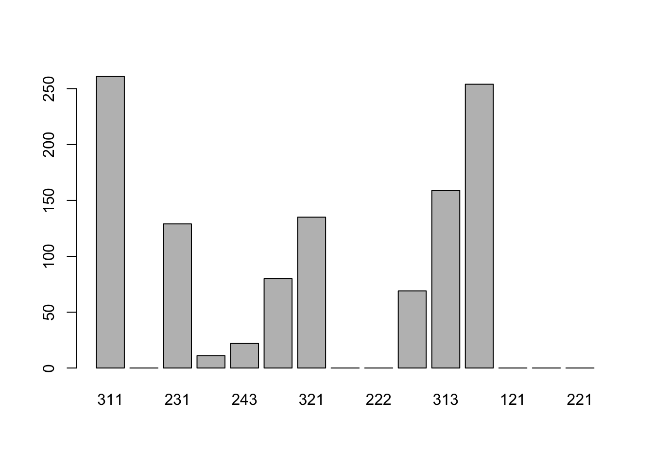
6 Data formatting
Please add ONE additional variable (column) that is based on one or more of the variables already in the data. This must be an ecologically relevant variable, for example human_population divided by dist_to_town is not an ecologically relevant variable, but the binary hunting variable from the cows data where years prior to hunting ban were coded as ‘1’ and years after hunting ban ‘0’ is an ecologically relevant variable generated from the existing data. You cannot use the hunting example as your variable, there are several possibilities here; you may want to use the information from your data exploration to inform this decision
bear_damage_tidy <-  bear_damage_tidy %>%

  # add new column that groups all forest types
  mutate(prop_forest = rowSums(across(c(prop_coniferous,
                                      prop_deciduous,
                                      prop_mixedforest))))


summary(bear_damage_tidy$prop_forest)
## Min. 1st Qu. Median Mean 3rd Qu. Max.
## 0.00 48.67 73.72 67.07 93.29 100.00# view(bear_damage_tidy)7 Fit some models
Create a candidate set of 8-10 models that represent hypotheses about what variables may explain your chosen response and fit these to a glm with the appropriate distribution
- Scale all numeric explanatory variables in your models
- One model must be a null model
- One model must include an interaction term AND have an appropriate
analog model without an interaction term to compare the relevance of the
interaction
- No global models (all non-correlated variables in one model)
Ensure these don’t include correlated variables and are not overparameterized
Check that these models are fitting appropriately before proceeding to question 7
# going to scale data first for ease of coding

bear_damage_tidy <- bear_damage_tidy %>%

  # use mutate to change all numeric variables to scaled
  mutate_if(is.numeric,
            scale)


# answers will vary - I've done 3 for demonstration

bear_null <- glm(damage ~ 1,
                 data = bear_damage_tidy,
                 family = 'binomial')

# interaction between distance to forest and distance to town (close to both town and forest would have high prob of damage)
bear_distance_i <- glm(damage ~ dist_to_forest * dist_to_town,
                       data = bear_damage_tidy,
                 family = 'binomial')

# quick check that this model fit
summary(bear_distance_i)
##
## Call:
## glm(formula = damage ~ dist_to_forest * dist_to_town, family = "binomial",
## data = bear_damage_tidy)
##
## Deviance Residuals:
## Min 1Q Median 3Q Max
## -2.7420 -0.7138 -0.5430 -0.2199 2.5861
##
## Coefficients:
## Estimate Std. Error z value Pr(>|z|)
## (Intercept) -1.1042 0.1433 -7.705 1.31e-14 ***
## dist_to_forest 1.6345 0.4750 3.441 0.00058 ***
## dist_to_town 0.2209 0.2179 1.014 0.31070
## dist_to_forest:dist_to_town 3.5312 0.7857 4.494 6.99e-06 ***
## ---
## Signif. codes: 0 '***' 0.001 '**' 0.01 '*' 0.05 '.' 0.1 ' ' 1
##
## (Dispersion parameter for binomial family taken to be 1)
##
## Null deviance: 1044.92 on 1119 degrees of freedom
## Residual deviance: 960.37 on 1116 degrees of freedom
## AIC: 968.37
##
## Number of Fisher Scoring iterations: 7# analog distance model w/o interaction
bear_distance <- glm(damage ~ dist_to_forest +
dist_to_town,
data = bear_damage_tidy,
family = 'binomial')
# quick check that this model fit
summary(bear_distance)##
## Call:
## glm(formula = damage ~ dist_to_forest + dist_to_town, family = "binomial",
## data = bear_damage_tidy)
##
## Deviance Residuals:
## Min 1Q Median 3Q Max
## -0.9293 -0.7004 -0.5669 -0.3137 2.3822
##
## Coefficients:
## Estimate Std. Error z value Pr(>|z|)
## (Intercept) -1.69548 0.09292 -18.247 < 2e-16 ***
## dist_to_forest -0.62093 0.18654 -3.329 0.000872 ***
## dist_to_town -0.62435 0.10685 -5.843 5.12e-09 ***
## ---
## Signif. codes: 0 '***' 0.001 '**' 0.01 '*' 0.05 '.' 0.1 ' ' 1
##
## (Dispersion parameter for binomial family taken to be 1)
##
## Null deviance: 1044.92 on 1119 degrees of freedom
## Residual deviance: 991.73 on 1117 degrees of freedom
## AIC: 997.73
##
## Number of Fisher Scoring iterations: 68 Model selection
Perform model selection on your candidate set of models and identify the best fit model/s
model.sel(bear_null,
          bear_distance,
          bear_distance_i)
## Model selection table
## (Int) dst_to_frs dst_to_twn dst_to_frs:dst_to_twn df logLik
## bear_distance_i -1.104 1.6340 0.2209 3.531 4 -480.183
## bear_distance -1.695 -0.6209 -0.6243 3 -495.865
## bear_null -1.538 1 -522.462
## AICc delta weight
## bear_distance_i 968.4 0.00 1
## bear_distance 997.8 29.35 0
## bear_null 1046.9 78.53 0
## Models ranked by AICc(x)9 Check model assumptions
This section will vary depending on the response variable you chose, variables you included in your models, etc. So I’m not specifying particular code to run, re-visit the GLM lab and other stats resources if needed to ensure you’ve answered the following question adequately with both code and a written response
- Check if your model violates any assumptions
- For each assumption have a brief annotation explaining what you’re testing and the conclusion you’ve drawn
If your model appears to violate any assumptions you don’t need to re-run it, just proceed
# check assumptions for top model

vif(bear_distance_i)
## there are higher-order terms (interactions) in this model
## consider setting type = 'predictor'; see ?vif## dist_to_forest dist_to_town
## 4.770770 3.652366
## dist_to_forest:dist_to_town
## 7.012544# plot VIF
vif(bear_distance_i) %>%
# Converts the named vector returned by vif() into a tidy tibble
enframe(name = 'Predictor',
value = 'VIF') %>%
# plot with ggplot
ggplot(aes(x = reorder(Predictor, VIF), # reorders from smallest VIF to largest (not sure I want like this)
y = VIF)) +
# plot as bars
geom_bar(stat = 'identity', fill = 'skyblue') +
# add labels
labs(x = 'Predictor',
y = 'VIF') +
# set theme
theme_classic()## there are higher-order terms (interactions) in this model
## consider setting type = 'predictor'; see ?vif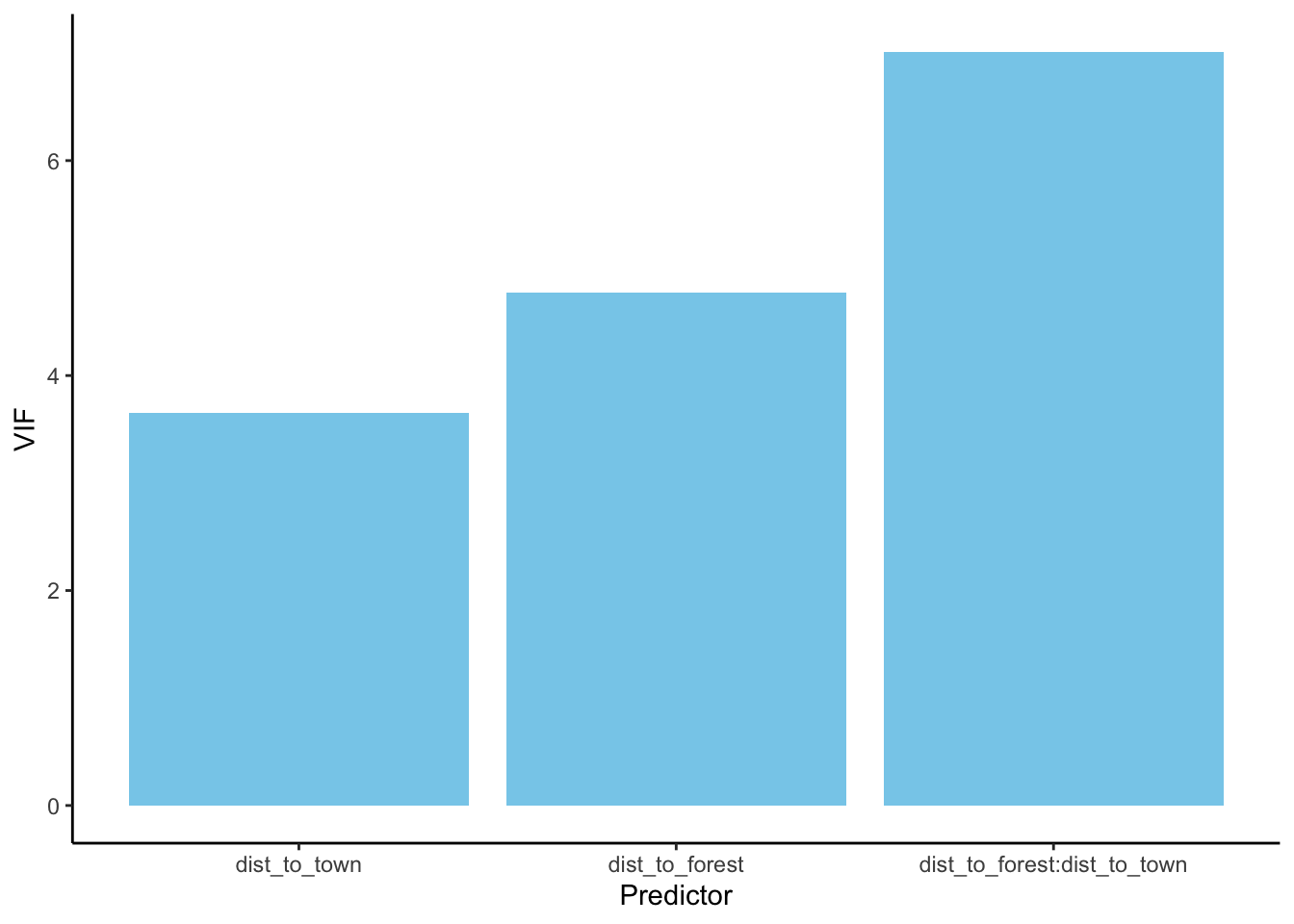
# dispersion
summary(bear_distance_i)
##
## Call:
## glm(formula = damage ~ dist_to_forest * dist_to_town, family = "binomial",
## data = bear_damage_tidy)
##
## Deviance Residuals:
## Min 1Q Median 3Q Max
## -2.7420 -0.7138 -0.5430 -0.2199 2.5861
##
## Coefficients:
## Estimate Std. Error z value Pr(>|z|)
## (Intercept) -1.1042 0.1433 -7.705 1.31e-14 ***
## dist_to_forest 1.6345 0.4750 3.441 0.00058 ***
## dist_to_town 0.2209 0.2179 1.014 0.31070
## dist_to_forest:dist_to_town 3.5312 0.7857 4.494 6.99e-06 ***
## ---
## Signif. codes: 0 '***' 0.001 '**' 0.01 '*' 0.05 '.' 0.1 ' ' 1
##
## (Dispersion parameter for binomial family taken to be 1)
##
## Null deviance: 1044.92 on 1119 degrees of freedom
## Residual deviance: 960.37 on 1116 degrees of freedom
## AIC: 968.37
##
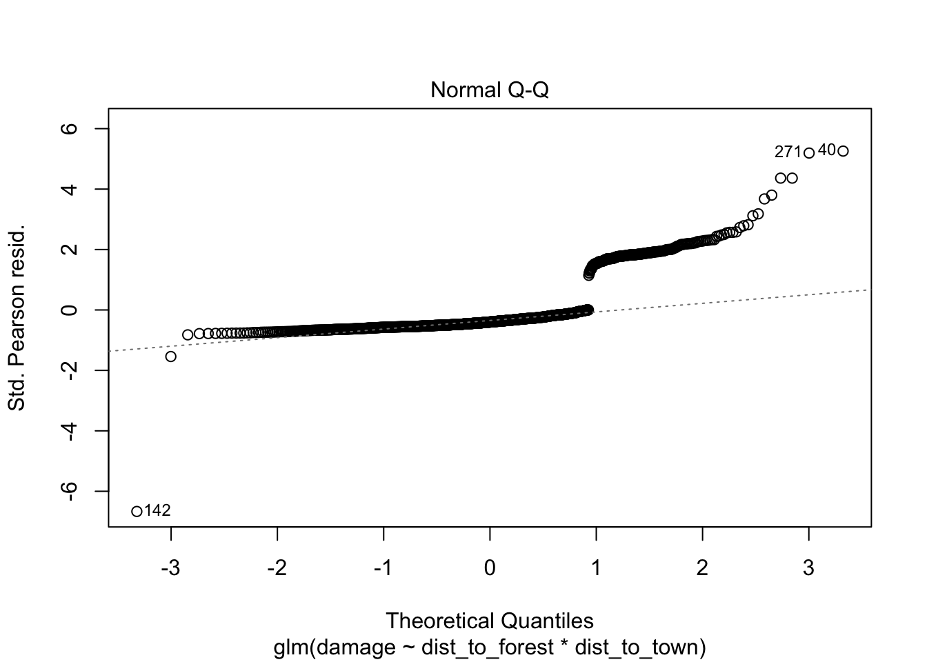
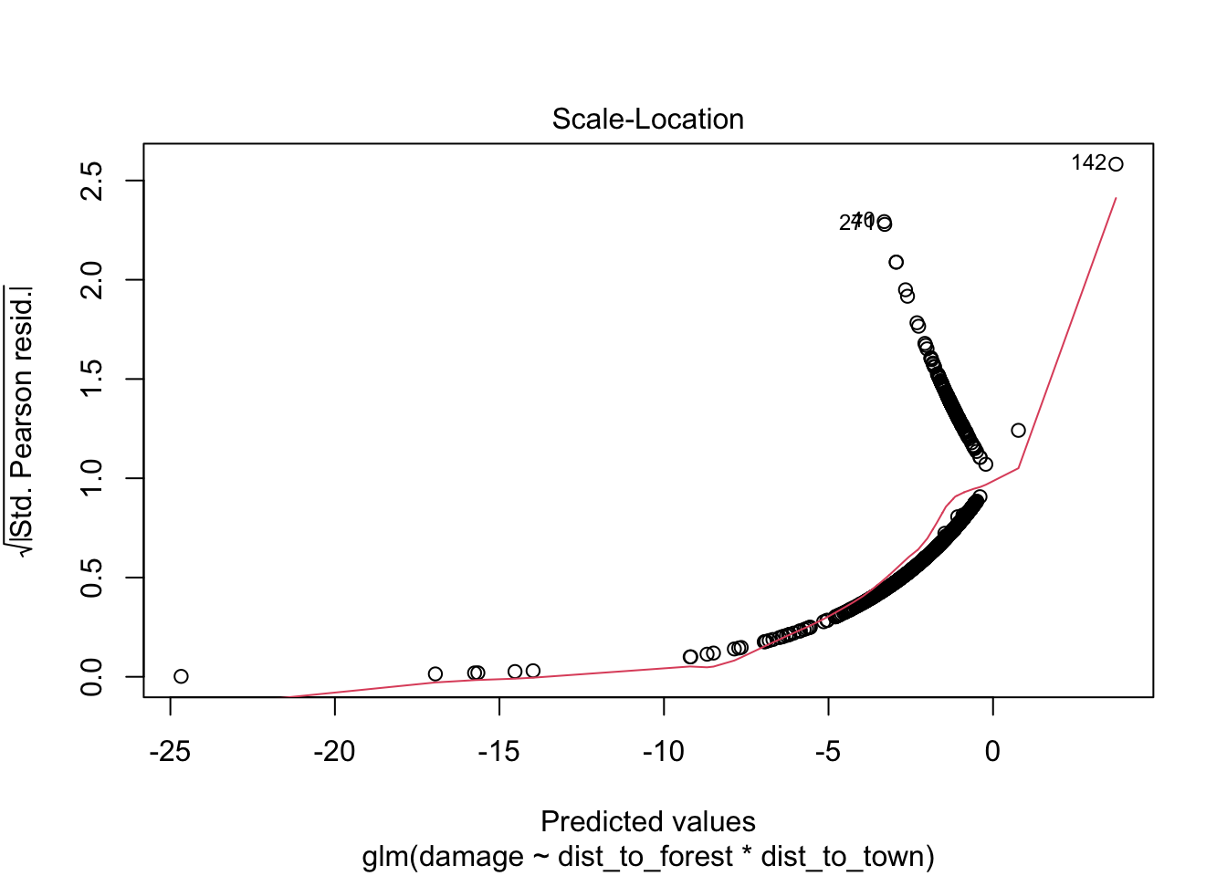
## Number of Fisher Scoring iterations: 7960.37/1116 # 0.86 slightly under dispersed but not a major issue for glm## [1] 0.8605466# check for observations with high leverage
plot(bear_distance_i) # ignore first three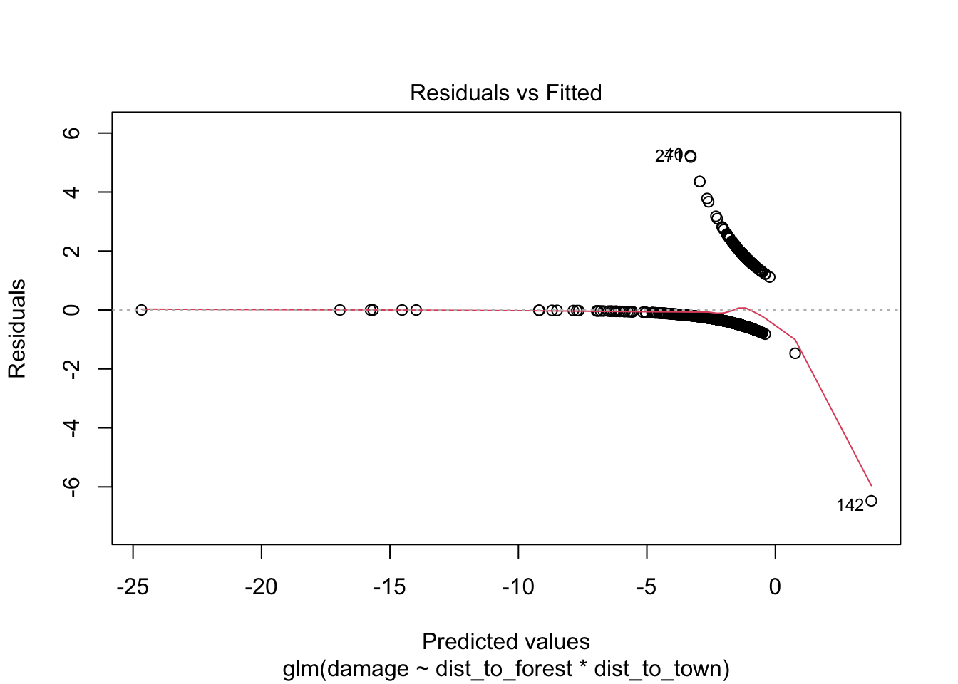
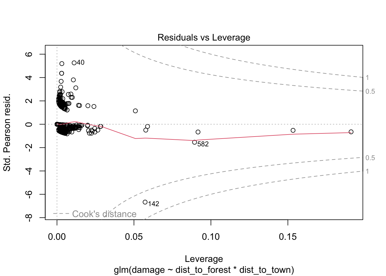 > VIFs are highish for individual terms which could indicate more
substantial violation of independence
> VIFs are highish for individual terms which could indicate more
substantial violation of independence
10 Interpret results
In bullet-point format provide annotations (comments) AND code (where necessary) that answer the following questions
- Do you have a singular best-fit model and why or why not?
- Was the interaction term useful? How do you know?
For your best-fit model (if you don’t have an obvious singular model pick one of the competitive models) and answer the questions below for that model:
- What variable/s best explain the variation in your response? How do
you know?
- Is this model a good fit to the data? How do you know?
11 Caveats
In bullet-point format provide annotations (comments) that speak to possible factors of the data, modeling approach, etc. which could contribute to uncertainty with your model selection, fit, and how you could improve this analysis